Latest Posts From Rafiul Hasan

Method 1 - Formatting Cells Between Time Range to Change Color Select the range of cells > go to the Home tab > click Conditional Formatting > ...

Protecting Excel cells means locking certain or all cells in the Excel worksheet to prevent any unwanted changes. In this free Excel tutorial, we will learn ...

In this article, you get a complete guideline of how to print an Excel sheet considering different aspects. Printing Excel sheets is an essential aspect of ...

Watch the Video – Create a Formula in Excel to Calculate Percentage Method 1 – Calculate the Percentage Formula to Compare Values We have a ...

How to Launch the VBA Editor in Excel Go to the Developer tab and select Visual Basic under Code. Alternative command: Pressing Alt + F11 will also ...

When working with large Excel worksheets, cleaning unnecessary data is essential. Deleting specific rows and shifting the remaining ones up to close the gap ...

In Excel VBA, the “While” loop is structured to repeat a block of code while a certain condition is true. The loop will continue executing until the condition ...

To compare one text with another in Excel, use Logical Operators. If one text is not equal to another in Excel, use the “Not Equal to” operator. Examples ...

Consider the dataset below. Some products of an online store, their order, and delivery dates are provided. Example 1 - Getting the Year, Quarter, ...

You may change the cell background color easily from the Home tab of the Excel worksheet by changing the Fill Color of a cell. But do you know that you can ...

Are you looking for ways to evaluate string as code with Excel VBA? Visual Basic for Applications (VBA) is a versatile programming language widely used for ...
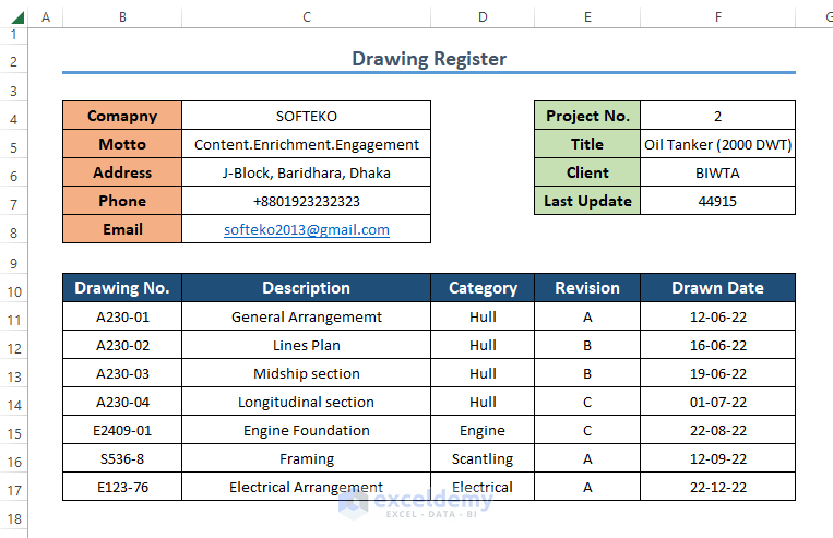
What Is a Drawing Register? A drawing register is essentially a list of drawings related to a project or a company. It includes essential details such as the ...
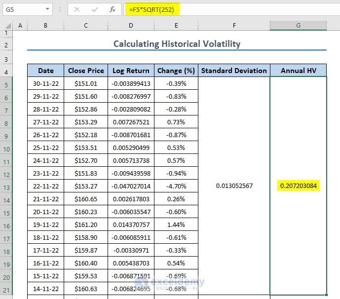
What Is Historical Volatility? In business aspects, the monetary value of different financial factors (i.e., stocks and currency) keeps fluctuating because of ...
![[Solved!] Excel Scaling Issues (2 Easy Methods)](https://www.exceldemy.com/wp-content/uploads/2022/12/Excel-Scaling-Issues-2.png?v=1697451704)
Method 1 - Change Scaling in Settings Steps: Go to the File tab from the Ribbon or press Ctrl + P. Select Print from the menu list, and the window ...
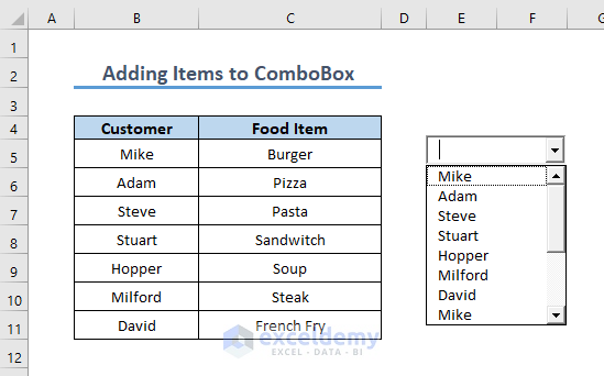
What Is a ComboBox in Excel? A ComboBox allows users to create or choose from a list of options. It is a type of a drop-down list based on a combination of ...
- « Previous Page
- 1
- 2
- 3
- 4
- …
- 8
- Next Page »
See Our Reviews at


Hi ROXANNE,
Thanks for your complement. The number 122 used for scaling is chosen based on empirical or trial-and-error methods to visually match the bell curve with the histogram in the specific context of this tutorial. It is not a standard or universally defined scaling factor; rather, it appears to be chosen to align the bell curve with the histogram in a way that the author finds visually pleasing or appropriate for his dataset. If you are reproducing this analysis for a different dataset, you may need to experiment with the scaling factor to achieve the best visual fit for your specific data. Adjusting this factor allows you to customize the appearance of the bell curve to better match the characteristics of your dataset.
Regards,
Rafiul Hasan
ExcelDemy
Hi,
You can use the following code. After sending mail for the first sheet, it will show message box for next sheet. Insert your ranges carefully for different sheets in the appeared input message box.
Regards
Rafiul Hasan
ExcelDemy
Hi AMY,
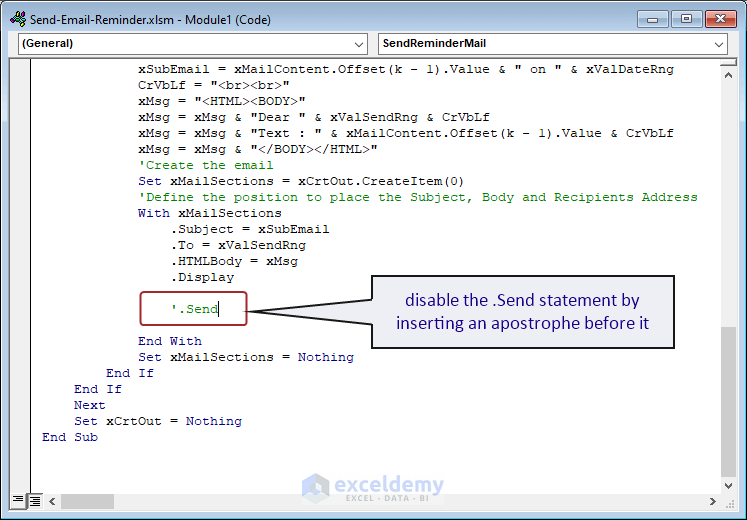
Most probably you haven’t disable the “.Send” statement in the VBA code. Disable the “.Send” statement by putting an apostrophe before it.
Regards
Rafiul Hasan
ExcelDemy
Hello JOHN,
Thanks for your comment. If new value is inserted in the range, the range changes (for example, from A2:A21 to A2:A25). You want to make the formula dynamic for the changed range. It seems you don’t want to use table. Actually, without using table, you won’t be able to make the formula dynamic.
The RANK function and the RANK.EQ function allow you to make the rank dynamic. But these functions assign the same rank to tied numbers and does not leave gaps in the ranking sequence. For example, if there is a tie for the second and third positions, both positions will be assigned a rank of 2, and the next distinct number will be ranked 4. But if you want to fill the next rank after ties, these functions are not useful. In that case, you have to use any of the methods stated in the article and copy the formula for the newly inserted value in the range. Without using table, it is not possible to make the formula dynamic.
Regards
Rafiul Hasan
Team ExcelDemy
Hi STEVE,
Thanks for your appreciation. And also sorry to hear that you faced difficulties with the 3rd method. I think you have faced problem in the GET.CELL function. Previously the sheet name (GET.CELL!) was also included in the formula and this may have occurred error. Actually there is no need to use the sheet name in the formula because Excel automatically updates the sheet name in the Name Manager. So, we have updated the formula to “
=GET.CELL(38,$D5)“. Try it and hope you will be able to make it now. Thanks again for your observation.Regards
Rafiul Hasan
Team ExcelDemy
Hi VLAD,
Thanks for your comment. You can checkout this article: How to Add Milestones to Gantt Chart in Excel.
Hope you find this helpful.
Regards,
Rafiul Hasan
Team ExcelDemy
Hi BAGUS,
In the context of Exponential Smoothing in Excel’s Data Analysis Toolpak, the Damping Factor refers to a parameter used to control the impact of older observations on the forecasted values.
The damping factor has a value between 0 and 1. It determines the weight assigned to the most recent observation when calculating the forecast. A higher value (closer to 1) gives more weight to the most recent data point, making the forecast more responsive to recent changes in the data. On the other hand, a lower value (closer to 0) gives less weight to the most recent data point, making the forecast more stable and less responsive to short-term fluctuations.
The value of Damping Factor being 0.91 suggests relatively high importance to the most recent data while still considering some historical data. The choice of 0.91 is somewhat arbitrary and depends on the specific characteristics of the data and the desired balance between responsiveness and stability in the forecast. Different values of the damping factor may be chosen based on the analyst’s judgment and the nature of the data being analyzed.
To determine the most appropriate value for the Damping Factor, it’s often a good practice to experiment with different values and evaluate the forecast accuracy using techniques like Mean Absolute Error (MAE) or Mean Squared Error (MSE). The choice of Damping Factor should ideally be data-driven and selected based on how well it performs in forecasting historical data or predicting future values.
Regards
Rafiul Hasan
Team ExcelDemy
Hi ANTHONEY,
Thanks for your comment. You requirement needs the Excel file. Please share your Excel file and repost your problem on our official ExcelDemy Forum. Our experts will try to reach you out.
Regards
Rafiul Hasan
Team ExcelDemy
Hi GREG,
I appreciate your suggestion. In VBA, there isn’t a built-in function to directly evaluate a string as code like in some other programming languages. You cannot directly evaluate a string as executable code like you would with the eval() function in JavaScript. Here, alternative approach has been provided to achieve similar results. You can achieve the concept of “evaluating strings as code” through code manipulation and dynamic formula evaluation. If you are looking for a method to directly execute arbitrary VBA code contained within a string, Excel VBA doesn’t provide a direct “eval” function for this purpose. The technique shared here provides structured way to achieve dynamic behavior in VBA.
Hello KRISTY,
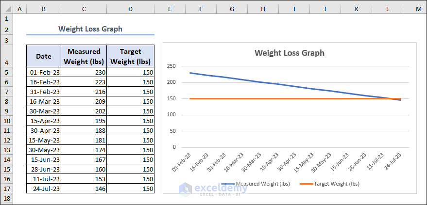
If you want to create a weight loss graph with values from 230 to 150, you’ll need to adjust the scale of the vertical (y-axis) to accommodate the new range. If you want to set your target weight as 150, you can create the weight loss graph in Excel like below:
Regards
Rafiul Hasan
Team ExcelDemy
Hello EDI,
the INDEX-MATCH formula can return a #VALUE! error under certain circumstances.
1. The MATCH function within the INDEX-MATCH formula couldn’t find a match for the lookup value in the specified array or range.
2. The INDEX function is expecting a numeric value as a result, but the matched value is non-numeric.
3. Incorrect arguments or ranges.
If you elaborate the problem you’re facing, then it will be easy to provide solution. Let us know if you face any difficulties.
Regards
Rafiul Hasan
Team ExcelDemy
Hi MASHAL,
You can use use VBA macro to automatically convert any entry you enter in specific cells to upper case by just only entering the text. Just follow these steps:
1. Press ALT + F11 to open the Visual Basic for Applications (VBA) editor.
2. In the Project Explorer window, locate and double-click on the “ThisWorkbook” module for the desired workbook.
3. In the appeared code window, paste the following code:
Replace “A1:Z100” with the range of cells you want to convert to uppercase.
4. Close the VBA editor.
Now, whenever you enter any text within the specified range, it will be automatically converted to uppercase without the need to manually run any macro. Adjust the range in the code as needed to match your desired cells.
Regards
Rafiul Hasan
Team ExcelDemy
Hi MARTIN PEREZ,
Thank you for your comment and for sharing your additional solution! I appreciate your input and the effort you put into finding a workaround for area chart markers. It sounds like you found an interesting method using a supporter series to manipulate the legend key font size. Your explanation will undoubtedly help other readers who come across your comment. Thank you again for your contribution!
Regards
Rafiul Hasan
Team ExcelDemy
Hi MARK,
Thanks for your comment. To learn different ways to print multiple sheets, you can follow this article of ExcelDemy: Print multiple sheets in Excel
If you want to print multiple sheets using VBA only, then follow this one: Print multiple Excel sheets to single PDF with VBA
Hope you will find this helpful.
Regards
Rafiul Hasan
Team ExcelDemy
Hi HANI,
Thanks for your query. The choice of epsilon depends on the desired accuracy of the eigenvalue estimate. It is typically a small positive value, and the algorithm terminates when the absolute difference between consecutive eigenvalue estimates falls below epsilon.
The specific value of epsilon will vary depending on the application and the desired level of accuracy. Using epsilon = 0.0005 indicates that the power method iterations will continue until the absolute difference between consecutive eigenvalue estimates falls below 0.0005. This level of tolerance can be suitable for many applications, especially when the eigenvalues of the matrix are relatively close in magnitude.
However, it’s important to note that the appropriate value of epsilon may vary depending on the specific problem and matrix being analyzed. If you find that the algorithm converges too quickly or does not reach the desired accuracy with epsilon = 0.0005, you may need to adjust the value accordingly.
Consider the scale and conditioning of the problem as well. If the matrix is ill-conditioned or has eigenvalues with large differences in magnitude, a smaller epsilon may be necessary to obtain accurate results.
So, it’s always important to assess the specific requirements of your problem and adjust the value of epsilon accordingly to achieve the desired accuracy.
Regards
Rafiul Hasan
Team ExcelDemy
Hi KEN,
This may encounter from several reasons.
1. If you have protected the worksheet or specific cells, it can prevent changes to the font settings. Try unprotecting the cells or the entire worksheet to see if that resolves the issue.
2. If there are any conflicting formatting applied to the cells, it might cause the barcode font to revert. Select the cells and clear any formatting such as bold, italic, or color changes. Then, set the font to “Code128” again.
3. Ensure that the page setup and print preview are correctly configured. Check the scaling options to make sure that the labels fit properly on the A4 sheet. Adjust the margins and other settings as needed to accommodate 51 labels per sheet.
4. If the above steps don’t solve the problem, try creating a new Excel file and follow the barcode printing steps from scratch. This can help identify if the issue is specific to your existing file.
Regards,
Rafiul Hasan
ExcelDemy Team
Hi ALLISON,
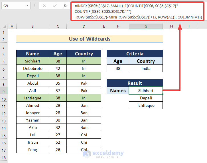
If you want to use wildcards with the second formula, you need to modify the dataset a little bit. Let’s say, we have short form of country name in the “Country” column. Our aim is to find the name of the person aged “38” and whose country is “India“. You can use the following formula:
=INDEX($B$5:$B$17, SMALL(IF(COUNTIF($F$6, $C$5:$C$17)*COUNTIF($G$6,$D$5:$D$17&”*”),ROW($B$5:$D$17)-MIN(ROW($B$5:$D$17))+1), ROW(A1)), COLUMN(A1))
We have used the wildcards character ampersand (*) in the second COUNTIF portion: COUNTIF($G$6,$D$5:$D$17&”*”)
As we want to find multiple output so it will result from an array. So, the $D$5:$D$17 acts as criteria as we can use wildcards character in criteria. This formula will match the short form mentioned in the country column and match it with criteria and extract the Name.
Hope you find this helpful.
Regards
Rafiul Hasan
Team ExcelDemy
Hi SINGGIH WAHYU N,
You can use VBA code for serving your requirement.
1. Select the merged cell(s) that contain data you want to copy.
2. Open the Visual Basic Editor by pressing Alt + F11.
3. Insert a new module by selecting “Insert” -> “Module” from the menu bar.
4. In the new module, enter the following code:
5. Run the code and a prompt will ask you to select the first cell of destination range. Select a cell where you want to paste values and you will get output.
Hope this help you. If you don’t want to use VBA, you have to first paste values and then use the “Go To Special” (pressing CTRL+G) dialog box and then select “Blanks”> click “OK” to remove blank cells.
Regards.
Rafiul Hasan
Team ExcelDemy
Hi DARRELL,
Congratulations on your new project. Be confident, you can make it. Based on your selections, you may use any of the following to get resulting list:
1. IF function: You can use the “IF” function to create a formula that checks if certain criteria are met and return the appropriate value. For example, if you have a pick list for materials and another for color, you can use an “IF” function to generate a list of materials that match the selected color.
2. VLOOKUP function: The “VLOOKUP” function can be used to search for a value in a table and return a corresponding value. You can set up a table with all the possible combinations of selections and use “VLOOKUP” to generate the resulting list based on the selections made.
3. FILTER function: The “FILTER” function can be used to filter a list based on certain criteria. You can set up a table with all the materials and their attributes (such as color, size, etc.) and use “FILTER” to generate a list of materials that match the selected attributes.
4. PivotTable: Pivot tables can be used to analyze and summarize data in a table. you can set up a table with all the selections made and your corresponding materials and use a pivot table to generate a list of materials based on the selections made.
These are just a few options you can consider. You will need to choose the one that works best for your specific situation. Don’t hesitate to contact with us if you face any problem. Best of luck.
Regards
Rafiul Hasan
Team ExcelDemy
Hi NOUR,
Thanks for the appreciation.
As per your requirement, it is possible to allow multiple users to access and edit a workbook on a network computer. Here are some steps you can follow in this regard:
1. Save your workbook on a shared network drive that all users have access to.
2. Restrict editing access for other users to ensure only authorized users can edit the workbook.
3. Create a login form that allows users to enter their credentials to access the userform. You can store user credentials in a separate worksheet within the workbook or use an external database.
4. Use VBA code to pull the necessary data from the shared workbook and display it to the userform.
5. When a user makes changes to the data in the userform, use VBA code to write the changes back to the shared workbook.
6. Implement a save feature that automatically saves changes made to the shared workbook when the userform is closed.
7. Create a backup plan to ensure data is not lost in case of system failure or network issues. This can include regular backups or saving a copy of the workbook in a secure location.
8. Test the userform with different user accounts to ensure it works as intended and all users can access and edit the shared workbook.
Hope this guide helps you to approach and solve the issue you’re facing. Actually it is not possible to give an exact solution without checking the Excel file. Most probably you need physical assistance in this regard. Let us know if you have any additional questions or concerns. You can also send your Excel file to our official mail address: [email protected]
Have a great day!
Regards
Rafiul Hasan | ExcelDemy Team
Hi DIEP TRAN,
The “Yes to all” button is a feature in Excel that allows you to apply a selected action to all the occurrences of the same conflict during a process. This button is usually available in the Name Manager dialog box, which pops up when you create, edit or delete names in your workbook.
The availability of the “Yes to all” button may vary depending on the version of Excel you are using. However, in most versions of Excel, including the latest version, which is Excel 2021, the “Yes to all” button should be available in the Name Manager dialog box.
If you are not seeing the “Yes to all” button in the Name Manager dialog box, it could be that the dialog box is not showing all the options. You can try expanding the dialog box to see if the “Yes to all” button is hidden or check your Excel settings to ensure that the option is enabled.
Overall, it’s best to consult the specific version of Excel you are using or refer to the documentation to learn more about the availability and functionality of the “Yes to all” button in Excel.
Regards
Rafiul | ExcelDemy Team
Hi JEFF,
Thanks for your concern. Actually, all the methods here explained are very easy to understand. Considering the situation, you have to choose the best-suited method for serving your purpose. If you don’t want to use any formula, then you can use Method 1.
Regards,
Rafiul | ExcelDemy Team
Hello AARON MWALE,
Thanks for your comment. Sorry to hear that you’re facing issues with Excel.
When Excel hangs and starts an Undo action, that means Excel is trying to process a large amount of data or executing a complex operation. This may cause the program to be unresponsive for a period of time while it completes the task.
In order to stop the undo action, you can try pressing the “Esc” key on your keyboard. If this does not work, you can try pressing “Ctrl” & “Break” on your keyboard. If don’t find these helpful, you may need to wait for Excel to finish the operation before you can regain control of the program.
To prevent Excel from hanging and starting an Undo action in the future, you can try the following:
1. Limit the amount of data you are working with at one time. If you are working with a large amount of data, try breaking it up into smaller chunks that are easier for Excel to handle.
2. Close any unnecessary programs or applications running in the background. This can free up system resources and improve Excel’s performance.
3. Disable any add-ins or macros that may be causing Excel to slow down or become unresponsive.
4. Check for and install any available updates for Excel. Updates often include bug fixes and performance improvements that can help prevent Excel from hanging in the future.
5. Consider upgrading your computer hardware if it is outdated or underpowered. Excel can be resource-intensive, and having a fast and capable computer can make a big difference in its performance.
Hope you find these ways helpful to overcome your issues.
Regards,
Rafi
ExcelDemy team
Dear BILLY,
Your PDF file should be readable in order to extract data. The application needs to recognize data. Please ensure a readable copy.
Regards
ExcelDemy Team
Hi TOM,
Thank you so much for letting us know. The formula has been edited. Thanks for your concern. Stay connected!
Regards,
Rafi
Author: ExcelDemy Team
Hello STEPH,
Did you enter any newer data into your pivot table field? With newer or re-entry of data, you need to go to the PivotTable Fields window (at the right corner of the worksheet)-> unmark the corresponding field of your data (i.e. Ship Date for this article) -> right-click on the PivotTable and click Refresh-> again mark the corresponding field that you unmarked a little bit ago.
Thanks and Regards
Hello SG,
You can customize the error message. In the Data Validation message box=> Error Alert icon, you can choose “Warning” style from the dropdown list. Now, if you try to input invalid data, the error message will show 3 options asking you whether you want to continue: Yes/No/Cancel/Help. Clicking “Yes” will allow you to proceed with the current value and will not show the error again.
Hello ANN HALL,
This may happen for different reasons.
1. Putting two statements in a single line. Check whether this is encountered and send the second statement in a new line.
2. Absence of parentheses.
3. Lack of whitespace in front of the ampersand(&) interpret as a long variable. So, put space between the variable and operator(&).
Hi KAREN LING,
Glad that you liked the template. This template has got fixed interest rate. You can add variable extra payments manually to your Excel file if you need it.
Regards,
Rafi (ExcelDemy Team)
Hi JON,
Thanks for your feedback. Can you please elaborate on your problem?
What I can say is that paying an extra amount from the minimum will reduce the next payments. You can proceed with your data. You can also share your Excel file with us and we will look into it.
Regards.
Rafi (ExcelDemy Team)
Hi ABDUS SALAM,
An equation is not like a formula as it isn’t supposed to perform any calculation. You can’t enter an equation in a particular cell in Excel just like you do for a formula. What you can do here is that, you can adjust height and width of the “Equation Editor” box or the cell as if it looks like the equation stays in the cell. This can serve your purpose to some extent.
Regards.
Hi KRISHNENDU,
Thanks for your comment. An equation is not like a formula as it isn’t supposed to perform any calculation. You can’t enter an equation in a particular cell just like you do for a formula. What you can do here is that, you can adjust height and width of your “Equation Editor” box or the cell as if it looks like the equation stays in the cell. I think this can serve your purpose to some extent.
Regards.