How to Use “Not Equal to” Operator for Text in Excel (5 Examples)

To compare one text with another in Excel, use Logical Operators. If one text is not equal to another in Excel, use the “Not Equal to” operator.

Examples are shown below:

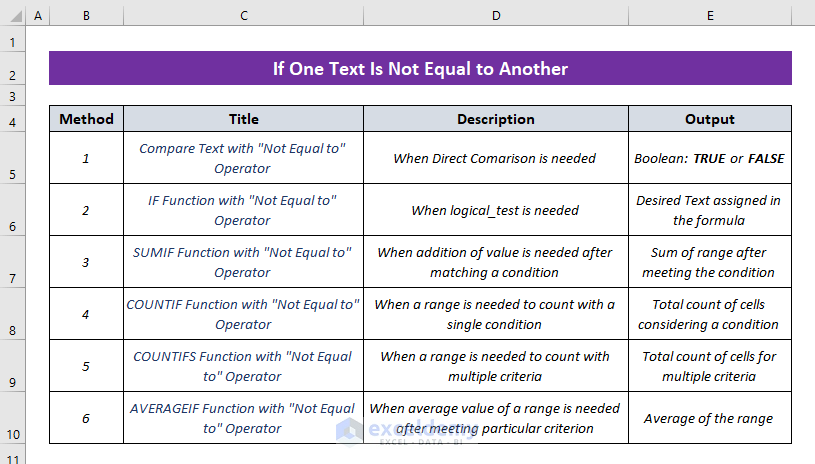
Introduction to “Not Equal to” Operator in Excel

The Not Equal to operator is used for comparing two values. Its function is opposite to the Equal (=) operator. Excel takes a pair of angle brackets (<>) as the Not Equal to operator. It returns a Boolean expression either TRUE (when not equal to) or FALSE (when equal to).

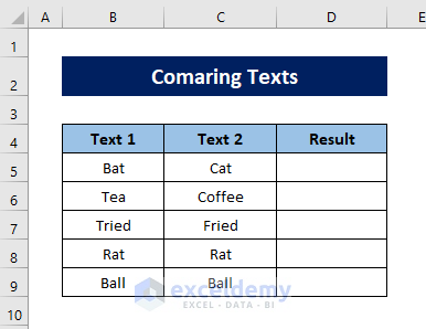
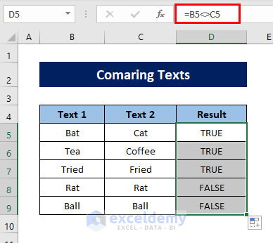
Method 1 – Compare a Text with Another Using “Not Equal to” Operator Directly

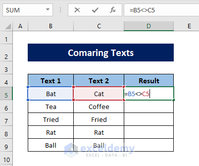
To compare Text 1 and Text 2 from this dataset:

⏩ Steps:

• Enter the following formula for comparing cells B5 and C5.

• Press ENTER and the cell will return TRUE as the text values of these two cells don’t match.
• Drag the Fill Handle tool downward to Autofill the formula below.

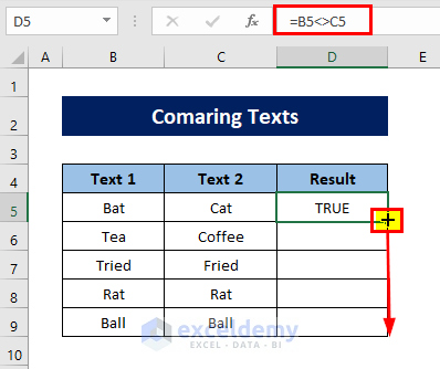
• The Boolean result will be shown after comparing all the text values.

Method 2 – Use of “Not Equal to” Operator in IF Function to Set a Logical Test

⏩ Steps:

• Apply the following formula to match cell B5 with C5.

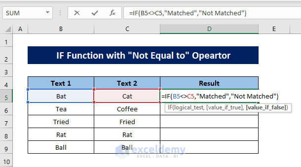
• Press ENTER and copy the formula down to the other cells. If the text values match, Excel will return “Matched” else “Not Matched”.

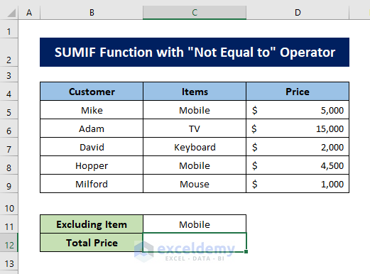
Method 3 – Apply “Not Equal to” Logic in SUMIF Function to Get Sum Excluding a Text Set Beforehand

To calculate the total price from this dataset excluding the item: Mobile.

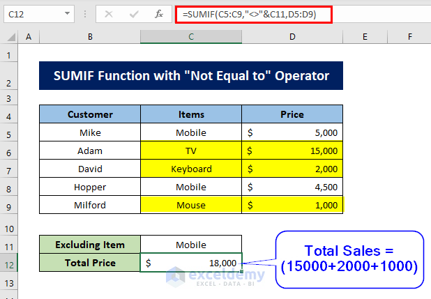
⏩ Steps:

• Enter the formula in cell C12.

• It will return the total price of the products excluding Mobile (i.e. 18000).

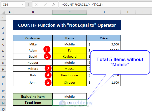
Method 4 – Using “Not Equal to” with COUNTIF and COUNITFS Functions

4.1 Single “Not Equal to” Criterion (COUNTIF Function)

⏩ Steps:

• Select a cell and add the formula below.

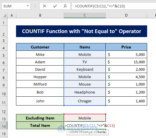
• Press ENTER to count the number of items excluding Mobile.

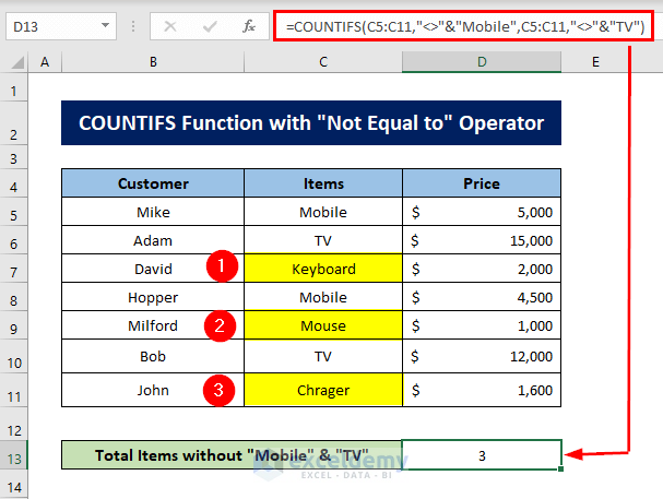
4.2 Multiple Simultaneous “Not Equal to” Criteria (COUNTIFS Function)

To count the items without “Mobile” and “TV”:

⏩ Steps:

• Apply the following formula in a selected cell.

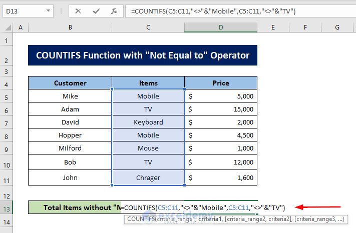
• Press ENTER to count the total cells excluding Mobile and TV.

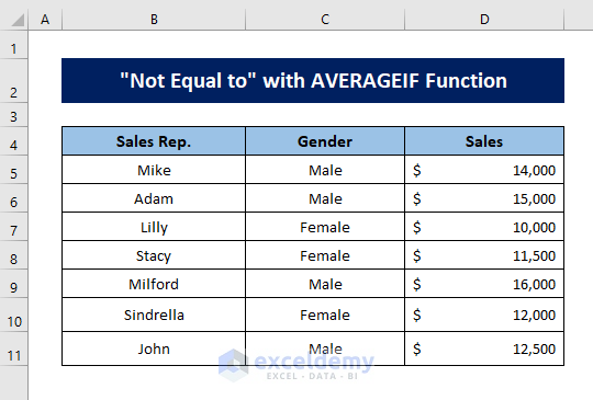
Method 5 – Use of “Not Equal to” Criteria with AVERAGEIF Function to Get Average Except for an Item

To find the average sales of Male and Female Sales reps respectively from the given dataset:

⏩ Steps:

• Apply the following formula to get the average sales by the Male sales reps.

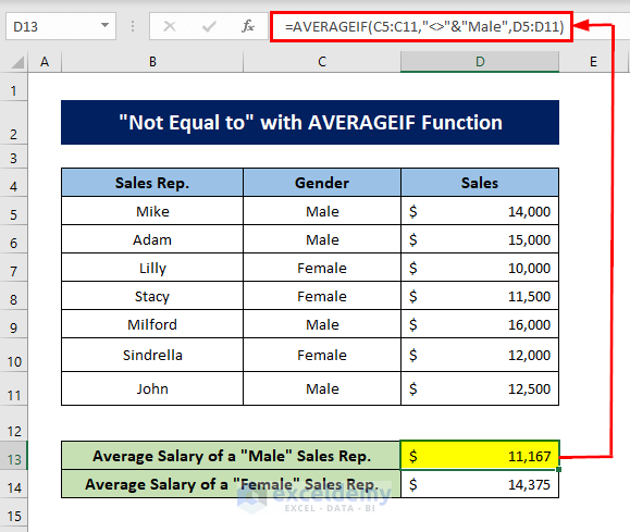
This formula will take the Male from the range C5:C11 and calculate the corresponding sales values from the range D5:D11 and calculate the average of the Male reps.

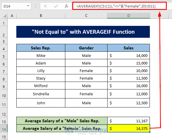
• To calculate the average of Female sales reps, apply the formula below.

Things to Remember

• The “Not Equal to” operator is not case-sensitive. So, if you have the same words with uppercase and lowercase (i.e. Rat and rat), it will return FALSE.
• You need at least two variables to apply this operator.

Download Practice Workbook

<< Go Back to Text | If Cell Contains | Formula List | Learn Excel