Here’s an overview of using the VLOOKUP function to get a partial case-insensitive match within an array.

How to Use VLOOKUP If a Cell Contains a Word within Text in Excel: 2 Ways
Method 1 – VLOOKUP to Find Data from Text Containing a Word in Excel
In the following picture, Column B contains the model names of several random chipsets and in Column C, there are names of the smartphone models which are using the mentioned chipsets. We’ll look for a partial match of a chipset model and we’ll extract which device uses this specified chipset.

- We’ll insert the partial match text in C13.
- Insert the following formula in the result cell C14 and press Enter.
=VLOOKUP("*"&C13&"*",B4:C11,2,FALSE)
Method 2 – VLOOKUP to Extract Data Based on a Value from a Particular Position in the Cell
Column B contains telephone numbers in different states. Columns D and E show the area codes and corresponding state names. We’ll copy a phone number from Column B and then find out the state name by extracting the code from the left 3 digits of the telephone number.
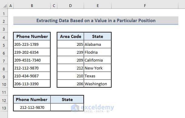
- The lookup value will be copied into B13.
- Insert the following formula in the result cell C13 and press Enter.
=VLOOKUP(VALUE(LEFT(B13,3)),D4:E10,2,FALSE)
An Alternative to VLOOKUP to Find Data Based on a Word within Text
The XLOOKUP function is the combination of VLOOKUP and HLOOKUP functions. It extracts data based on the inputs of the lookup array and returns the array. The generic formula of this function is as follows:
=XLOOKUP(lookup_value, lookup_array, return_array, [if_not_found], [match_mode], [search_mode])
- Based on the first dataset in Method 1, the required formula in the output Cell C14 should look like this:
=XLOOKUP("*"&C13&"*",B4:B11,C4:C11,"Not Found",2)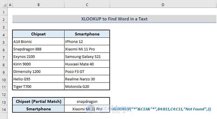
The fourth argument contains a customized message that will be shown if the lookup value is not found in the table. The fifth argument (match_mode) has been defined by ‘2’ which denotes wildcard match based on the input in the first argument.
Download the Practice Workbook
<< Go Back to Text | If Cell Contains | Formula List | Learn Excel
Get FREE Advanced Excel Exercises with Solutions!

is it possible to do something like put “A14, Snapdragon” as the lookup word in one cell and the function would reply list of all possible lookup results “iPhone 12, Xiaomi Mi 11 Pro” also in one cell.
Hello, Thomas!
You can apply the following formula in cell C14 to do that.
=TEXTJOIN(", ",,(VLOOKUP(LEFT(C13,(FIND(",",C13,1)-1))&"*",B5:C11,2)), (VLOOKUP(TRIM(RIGHT(C13, LEN(C13)-FIND(",",C13,1))&"*"), B5:C11,2)))**Notes:
1. If multiple results are associated with the lookup value, the formula will return the first result only.
2. You must enter at least 2 lookup values separated by comma. Otherwise, you may see #VALUE!
Regards
Shamim
Is it possible to do a lookup with the search key being something along the lines of AMZN234567 and the range has just AMZN? im trying to easily categorize expenses, and i want to create a rule where it looks in the expense description for certain terms in the description, such as finding a partial match of AMZN in the AMZN234567 description, and bring in the budget category mapping, something like ‘office supplies’ which will sit in another data table. How can i do that? it sounds like i would need a fuzzy lookup, but am unsure. Thanks!
Hello BEN!
I think the solution to your problem is already solved in method 1 of this article. To search for partial match, you have the wild cards (*) that have been shown in method 1.
If the cell C13 contains the value of the search item. Then use the following formula:
=VLOOKUP(“”&C13&””,$B$4:$C$11,2,FALSE)
I hope, your problem will be solved in this way. If not, please share the Excel file and send us the problem with little more explanation in an email at [email protected]
Thank You!
Is it possible to do this search but the opposite way around. for example the search item is snapdragon 888 and it is looking for snapdragon in the lookup list?
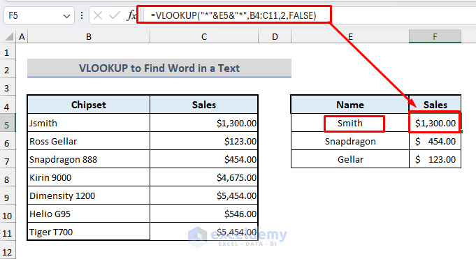
I have a set of data where people have entered their names i cannot change or set the format in which they enter them is it not my system but i want to pull data matching their surname to there department.
For example user enters J Smith or John Smith or JSmith but in my table i have smith and looking to return the value of “sales”
Hello Julie Binks,
Based on your table you can match data to return sales. Use the following formula to get data based on partial name.
=VLOOKUP(“*”&E5&”*”,B4:C11,2,FALSE)
Here is the sample data with output:
Regards
ExcelDemy
can this be done the other way around, like looking for “Jsmith” but wanting to find “Smith”?
Hello TV,
Yes, it is possible to do it the other way around where your lookup value is “JSmith” and you want to match “Smith” from the table.
You can achieve this by checking if any of the words in your lookup value contain a word from the lookup list. This requires an array formula (or FILTER/XLOOKUP in modern Excel) that checks if each entry in the table is contained within your search term.
Here’s an example using FILTER:
=FILTER(C2:C11, ISNUMBER(SEARCH(B2:B11, E5)))
1. E5 is your input (like “JSmith”)
2. B2:B11 contains your surnames (like “Smith”)
3. C2:C11 contains departments (like “Sales”)
This formula returns the department(s) whose name exists inside the input like “JSmith”.
Regards
ExcelDemy
Hello,
Is it possible to find a keyword within a string of phrases in one cell, but only have the returned value be the word within the string?
Example:
India is the lookup value, checking a cell where the string is ” 256 Indian Drive.” I would want my return value to only be the word “Indian.”
Thanks!
Hello Ryan,
Yes, it’s possible to achieve this in Excel! You can use a combination of formulas to extract the matching word from a string.
1. Use the SEARCH function to locate the position of your keyword within the string.
2. Use the MID function to extract the word based on the position.
If your lookup value is in cell A1 (e.g., “India”) and the text string is in B1 (e.g., “256 Indian Drive”), you can use the following formula:
=IF(ISNUMBER(SEARCH(A1,B1)),TRIM(MID(B1,SEARCH(A1,B1),LEN(A1))),”Not Found”)
This will return “Indian” if the word contains the keyword “India.” Adjust as needed for more specific cases.
Let me know if you’d like further clarification!
Regards
ExcelDemy
What if you have a list of terms that you are looking for, and you want to find one of them within a text, and return that term as a lookup, how would you do that?
i.e. you have the following text line “123 Blue Ridge Street”, but you have a list of terms that you’re looking for:
List of terms
Blue
Red
India
Mary
View
Black
How do you return “Blue” from the text above looking up from the list of terms provided?
Hello Tom,
You can use a combination of Excel functions to achieve this. Here’s a formula approach using FILTER and SEARCH:
Assume your list of terms is in cells A2:A7 and your text line is in B2 (“123 Blue Ridge Street”).
Formula:
=FILTER(A2:A7, ISNUMBER(SEARCH(A2:A7, B2)))
This will return “Blue” if it’s present in the text line.
Explanation:
1. SEARCH(A2:A7, B2) looks for each term in the text and returns a number if it finds a match.
2. ISNUMBER() checks if the result is a number, indicating a match.
3. FILTER() returns the matching term(s).
Regards
ExcelDemy