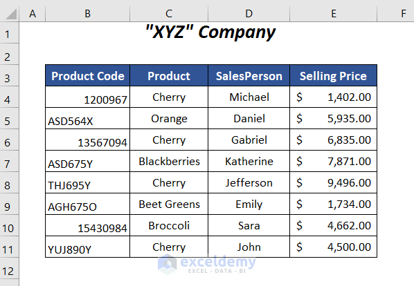
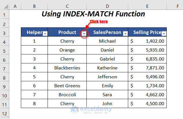
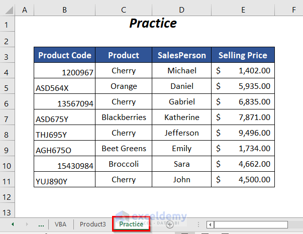
The following dataset contains records of product codes, product lists, salesperson’s names, and corresponding sales values for a company. Using this dataset, we will demonstrate how to copy the values of the corresponding cells if they contain text.
Method 1 – Using the Filter Option for Any Text Strings
Steps:
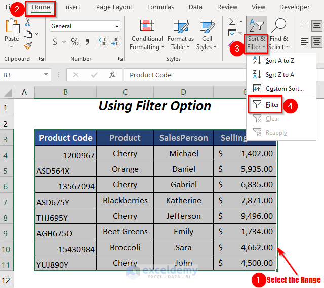
- Select the dataset and go to the Home Tab >> Editing Group >> Sort & Filter Group >> Filter Option.
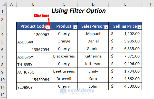
The Filter option will be enabled for this range.
- Click on the Filter drop-down symbol of the Product Code column.
- Select the Text Filters option and then the Custom Filter option.
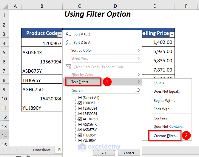
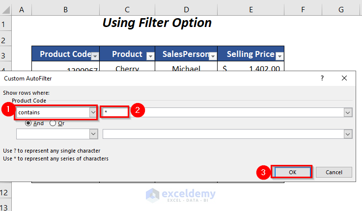
The Custom AutoFilter dialog box will open.
- Select the contains option in the first box,
- Enter the symbol (*) in the second box to allow text only.
- Press OK.
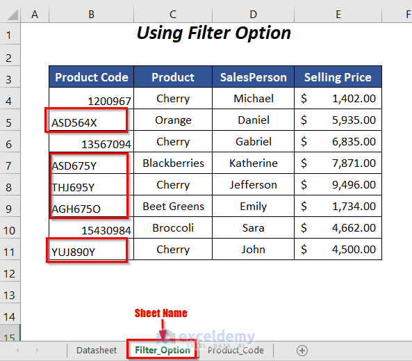
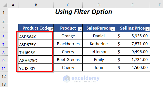
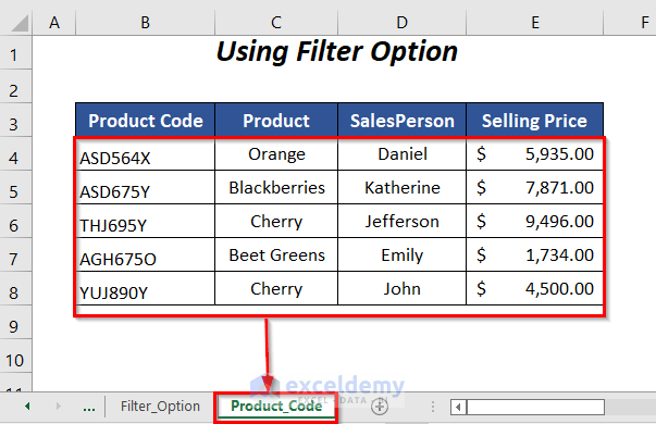
You will get the text product codes and their corresponding values.
- Press CTRL+C to copy the visible values of the dataset, and then go to the new sheet Product_Code.
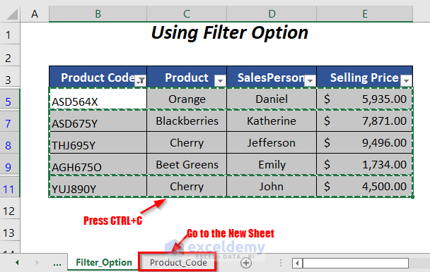
- Select cell B4 of the new sheet where you want to paste the values and press CTRL+V.
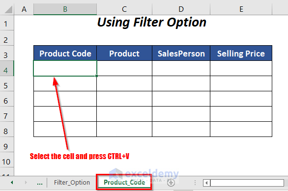
You will get the product codes in text format and their corresponding values in the new sheet Product_Code.
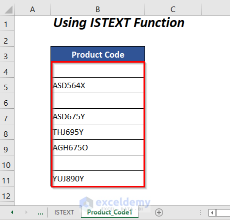
Method 2 – Using the ISTEXT Function
Steps:
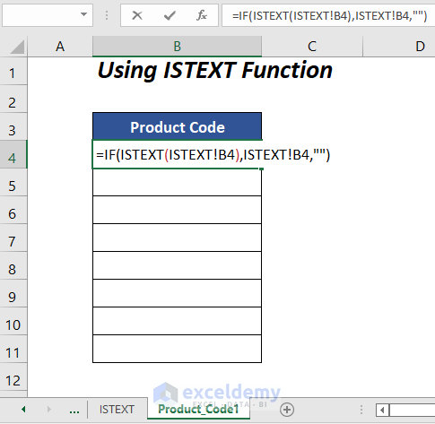
- Enter the following formula in cell B4 of the sheet Product_Code1.
=IF(ISTEXT(ISTEXT!B4),ISTEXT!B4,"")Here, ISTEXT!B4 is the Product Code in cell B4 of the ISTEXT sheet. ISTEXT will check if the cell value is text; if it is text, then IF will return this value; otherwise, it is blank.
- Press ENTER and drag down the Fill Handle tool.
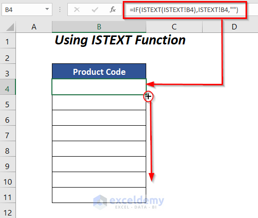
You will get the following product codes in text format in the new sheet Product_Code1.
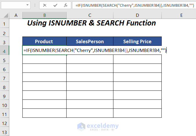
Method 3 – Using the ISNUMBER and SEARCH Functions
Steps:
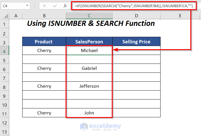
- Enter the following formula in cell B4 of the sheet Product_Name:
=IF(ISNUMBER(SEARCH("Cherry",ISNUMBER!B4)),ISNUMBER!B4,"")Here, ISNUMBER!B4 is the Product Code in cell B4 of the ISNUMBER sheet.
SEARCH("Cherry",ISNUMBER!B4)becomes
SEARCH("Cherry", "Cherry")→ returns the number of the character at which the given text string is found first.
Output → 1
ISNUMBER(SEARCH("Cherry",ISNUMBER!B4))becomes
ISNUMBER(1)→ returns TRUE for numbers otherwise FALSE
Output → TRUE
IF(ISNUMBER(SEARCH("Cherry",ISNUMBER!B4)),ISNUMBER!B4,"")becomes
IF(TRUE,"Cherry","")→ returns Cherry for TRUE otherwise blank
Output → Cherry
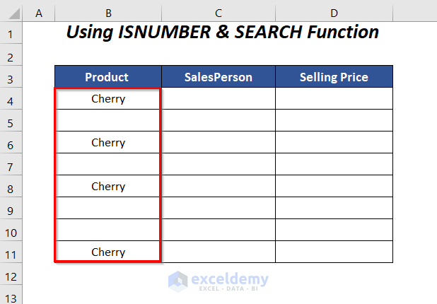
- Press ENTER and drag down the Fill Handle tool.
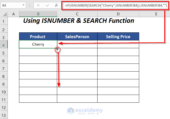
You will get the text string Cherry and blanks for other products in the Product column.
- To get the corresponding salesperson’s name in the SalesPerson column, enter the following formula:
=IF(ISNUMBER(SEARCH("Cherry",ISNUMBER!B4)),ISNUMBER!C4,"")To meet the criterion, it will return the value of cell C4 of the ISNUMBER sheet.
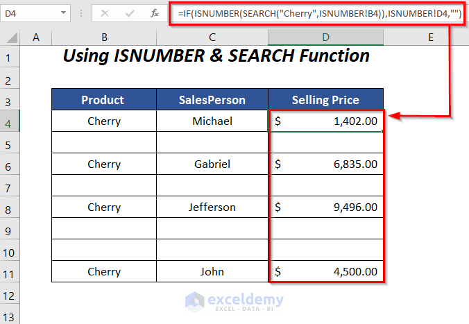
- To extract the selling prices, use the following formula:
=IF(ISNUMBER(SEARCH("Cherry",ISNUMBER!B4)),ISNUMBER!D4,"")To meet the criterion it will return the value of cell D4 of the ISNUMBER sheet.
Method 4 – Using the FILTER Function
Steps:
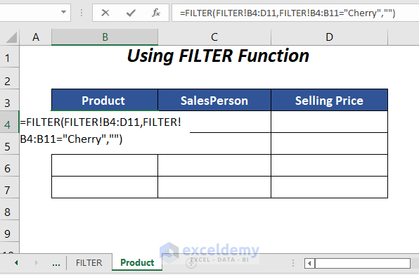
- Enter the following formula in cell B4 of the sheet Product.
=FILTER(FILTER!B4:D11,FILTER!B4:B11="Cherry","")Here, FILTER!B4:D11 is the range of the FILTER sheet; then FILTER will search for the value Cherry in the range FILTER!B4:B11, and for empty cells, it will return a blank.
- Press ENTER to get the salespersons’ names and the sale values for the product Cherry.
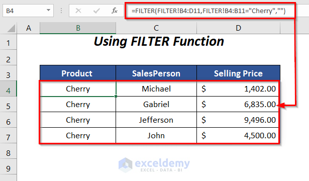
Note: The FILTER function is only available for Microsoft Excel 365 version.
Method 5 – Using the INDEX and MATCH Functions
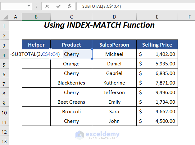
5.1 Getting Updated Serial Numbers with the Help of the SUBTOTAL Function
- Enter the following formula in cell B4:
=SUBTOTAL(3,C$4:C4)Here, 3 is for the COUNTA function, and C$4:C4 is the range that will be updated for each successive row. For example, Row 8 will be C$4:C8 because we have fixed the first limit by putting a $ symbol before Row 4.
- Press ENTER and drag down the Fill Handle tool.
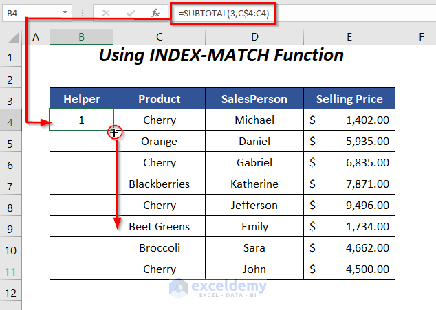
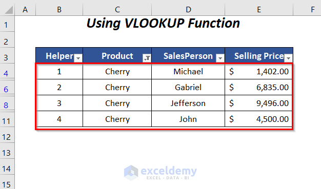
You will get the serial numbers in the Helper column.
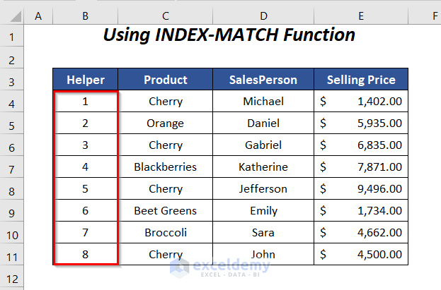
We will enable the filter option for this range.
- Select the dataset and then go to the Home Tab >> Editing Group >> Sort & Filter Group >> Filter Option.
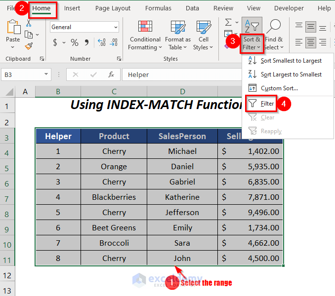
You will enable the Filter option for this range.
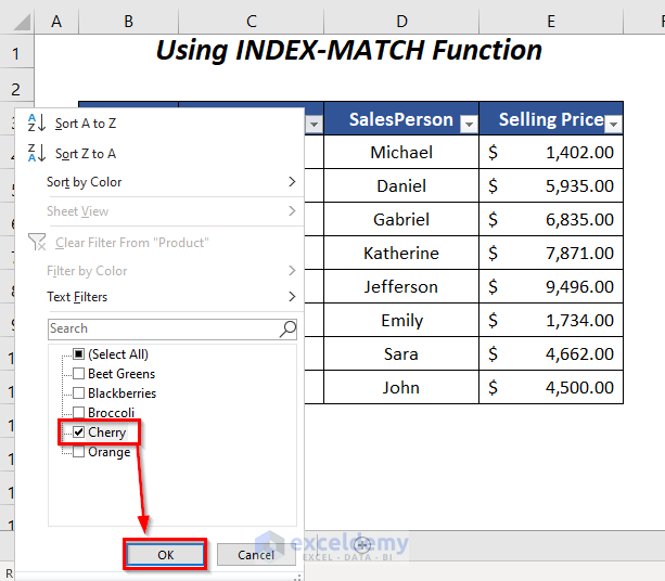
- Click on the Filter drop-down symbol of the Product column.
- Check only the product Cherry from the drop-down list of the Product column and press OK.
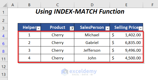
You will get the filtered table and see the serial numbers are automatically updated from 1 to 4.
5.2 Using the Combination of INDEX and MATCH Functions to Extract the Values
- Go to the new sheet Product1 and write down the serial numbers in the Serial No. column.
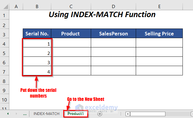
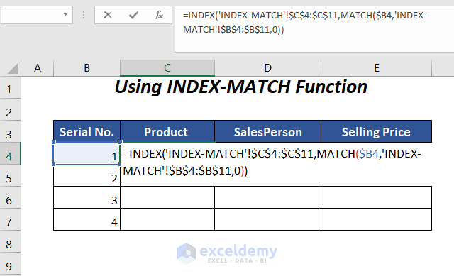
- Enter the following formula in cell C4:
=INDEX('INDEX-MATCH'!$C$4:$C$11,MATCH($B4,'INDEX-MATCH'!$B$4:$B$11,0))Here, ‘INDEX-MATCH’!$C$4:$C$11 is the range of the SalesPerson column in the INDEX-MATCH sheet from which we want to get the corresponding value, $B4 is the serial number which will match with the numbers in the range ‘INDEX-MATCH’!$B$4:$B$11 of the Helper column.
MATCH($B4,'INDEX-MATCH'!$B$4:$B$11,0)→ returns the row index number of the value in cell $B4, which is 1.
Output → 1
INDEX('INDEX-MATCH'!$C$4:$C$11,MATCH($B4,'INDEX-MATCH'!$B$4:$B$11,0))becomes
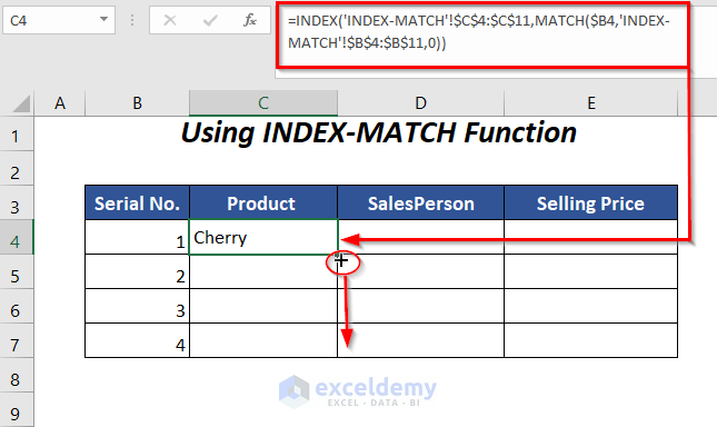
INDEX('INDEX-MATCH'!$C$4:$C$11,1)→ checks the corresponding value in the range $C$4:$C$11 for row index number 1
Output → Cherry
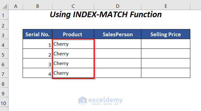
- Press ENTER and drag down the Fill Handle tool.
You will get the text strings, Cherry, from the old sheet to this new sheet.
- To extract the corresponding salesperson’s names for the product Cherry by entering the following formula:
=INDEX('INDEX-MATCH'!$D$4:$D$11,MATCH($B4,'INDEX-MATCH'!$B$4:$B$11,0))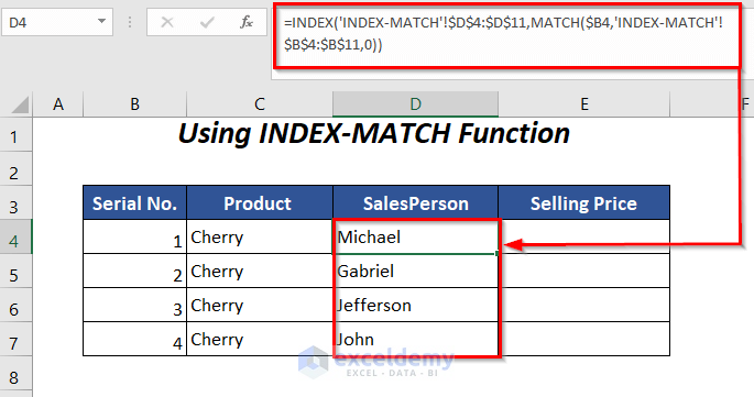
- To get the selling prices of the text string Cherry, enter the following formula:
=INDEX('INDEX-MATCH'!$E$4:$E$11,MATCH($B4,'INDEX-MATCH'!$B$4:$B$11,0))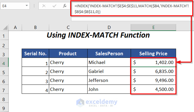
Method 6 – Using VLOOKUP
Steps:
➤ Follow section 5.1 to get the filtered table with updated serial numbers.
To copy these values to the new sheet Product, go to this sheet first.
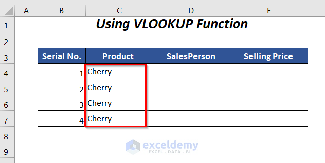
- Enter the serial numbers in the Serial No. column.

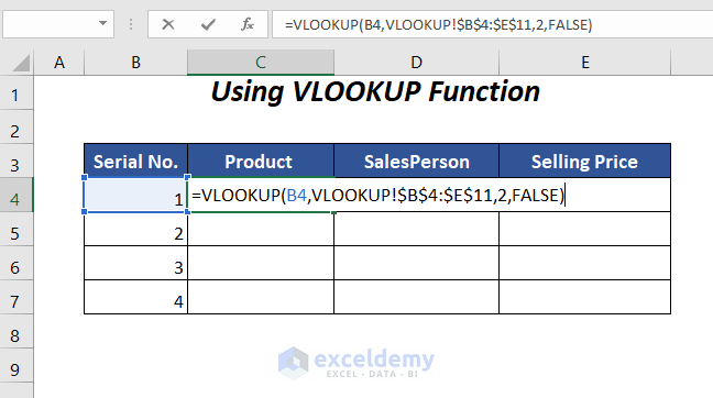
- Enter the following formula in cell C4:
=VLOOKUP(B4,VLOOKUP!$B$4:$E$11,2,FALSE)B4 is the lookup value, VLOOKUP!$B$4:$E$11 is the range in the VLOOKUP sheet where we will search for the lookup value and extract our desired value, 2 is the column index number of this range from which we will extract the Product names and FALSE is for an exact match.
- Press ENTER and drag down the Fill Handle tool.
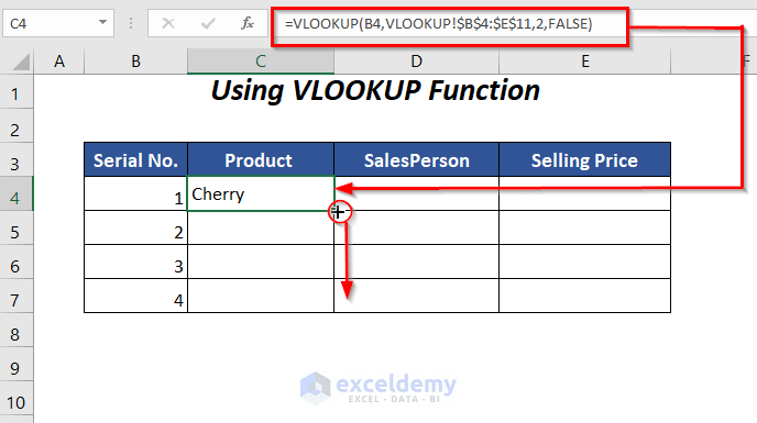
You will get the text strings, Cherry, from the old sheet to this new sheet.
- To get the corresponding salesperson’s name in the SalesPerson column, enter the following formula:
=VLOOKUP(B4,VLOOKUP!$B$4:$E$11,3,FALSE)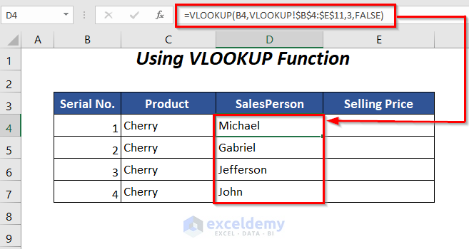
- To get the selling prices, enter the following formula:
=VLOOKUP(B4,VLOOKUP!$B$4:$E$11,4,FALSE)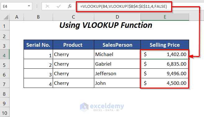
Method 7 – Using a VBA Code in Excel
Steps:
- Go to the Developer Tab >> Visual Basic Option.
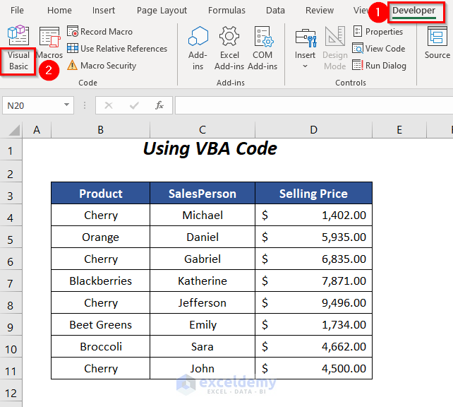
The Visual Basic Editor will open up.
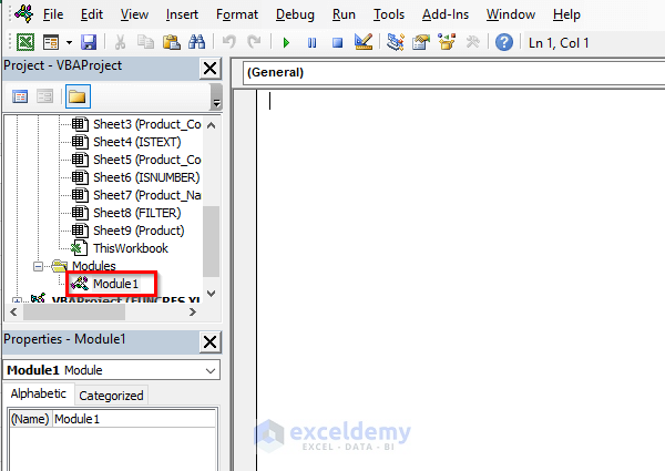
- Go to the Insert Tab >> Module Option.
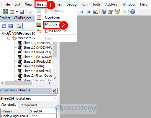
The Module will be created.
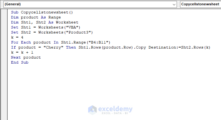
- Enter the following code:
Sub Copycellstonewsheet()

Dim product As Range
Dim Sht1, Sht2 As Worksheet
Set Sht1 = Worksheets("VBA")
Set Sht2 = Worksheets("Product3")

k = 4
For Each product In Sht1.Range("B4:B11")
If product = "Cherry" Then Sht1.Rows(product.Row).Copy Destination:=Sht2.Rows(k)
k = k + 1
Next product

End Sub
Here, we have declared the product as Range, which will be assigned to each cell value of the Product column, and Sht1 and Sht2 as Worksheet. We have set Sht1 to the old sheet VBA, Sht2 to the new sheet Product3.
The FOR loop will search for the text string Cherry in each cell of the B4:B11 range of Sht1; the IF-THEN statement will copy the corresponding rows if the cell in the Product column of this row contains Cherry. Paste it to the new sheet.
Here, k is determining the row number where we are pasting the values starting from 4 and incremented by 1.
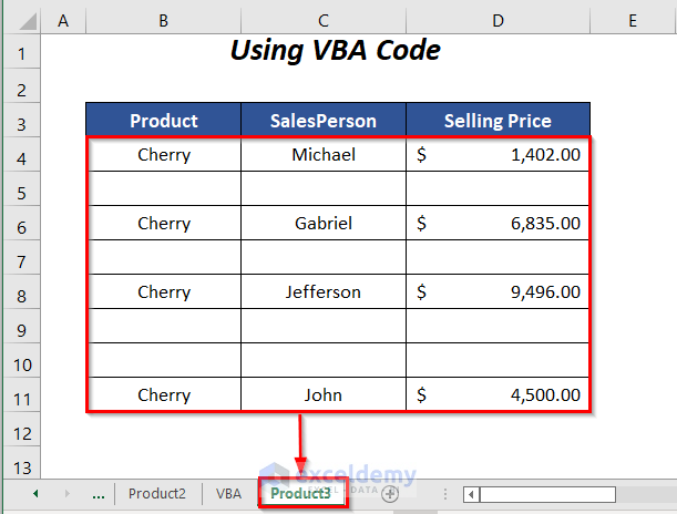
- Press F5.
The new sheet Product3 will contain the product Cherry, its corresponding Salesperson’s names, and Selling Prices.
Practice Section
For practicing by yourself, we have provided a Practice section.
Download the Workbook
<< Go Back to Text | If Cell Contains | Formula List | Learn Excel
Get FREE Advanced Excel Exercises with Solutions!
