In Excel, we often need to do various types of mathematical calculations. Anchoring columns is a common practice when performing these calculations. In this article, we will discuss two simple yet efficient methods for anchoring columns in Excel. So, let’s start this article and explore these methods.
What Is Anchoring?
Anchoring is a feature of Microsoft Excel that allows us to fix the reference of a cell or a range of cells in an Excel formula. The anchored cell references don’t change when we copy down the formula. This allows us to save a lot of time, as we don’t need to write the same formula again and again. Simply, we need to anchor the cell and copy down the formula to as many cells as we need.
Anchoring Columns in Excel: 2 Efficient Ways
In this section of the article, we will learn two simple methods for anchoring columns in Excel. Let’s say, we have the Daily Wages Comparison of 2 Companies as our dataset. Our goal is to calculate the Daily Wages for two different Hourly Wage rates by anchoring columns.

Not to mention, we used the Microsoft Excel 365 version for this article; however, you can use any version according to your preference.
1. Using Keyboard Shortcut for Anchoring Columns
Using the keyboard shortcut is the simplest way for anchoring columns in Excel. Let’s follow the steps mentioned below to do this.
Steps:
- Firstly, in cell D5, type in equal (=) and select cell C5.
- Then, press the F4 key from your keyboard three times. This will anchor column C.
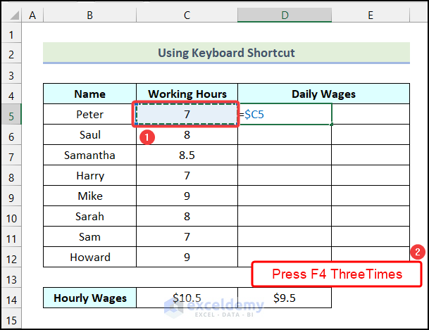
- Following that, enter a multiplication operator (*) and then select cell C14.
- Next, press F4 key two times. Doing this will anchor row 14.

Your final formula will be like this.
=$C5*C$14Here, cell C5 indicates the first cell of the Working Hours column, and cell C14 refers to the Hourly Wages for the first company.
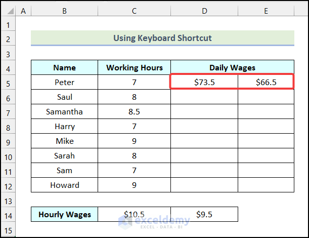
- Now, press ENTER.

As a result, you will have the following output on your worksheet.

- Then, drag the Fill Handle horizontally up to cell E5 and you will get the Daily Wages of Peter for two Hourly Wages rates.
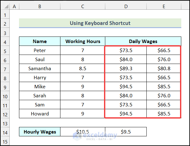
- Finally, use the AutoFill option of Excel to get the rest of the outputs as demonstrated in the following image.
2. Utilizing Excel VBA to Anchor Columns
Utilizing the VBA Macro feature is another smart way for anchoring columns in Excel. In the VBA code, we will use the R1C1 notation. Now, let’s use the instructions outlined below to do this.
Steps:
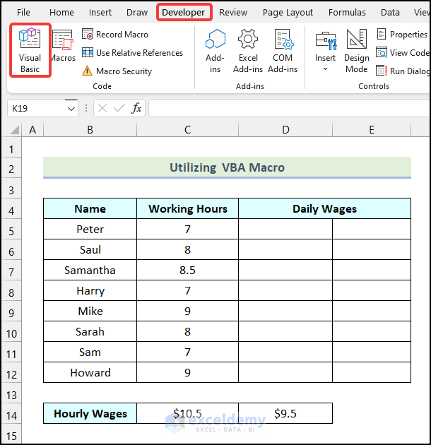
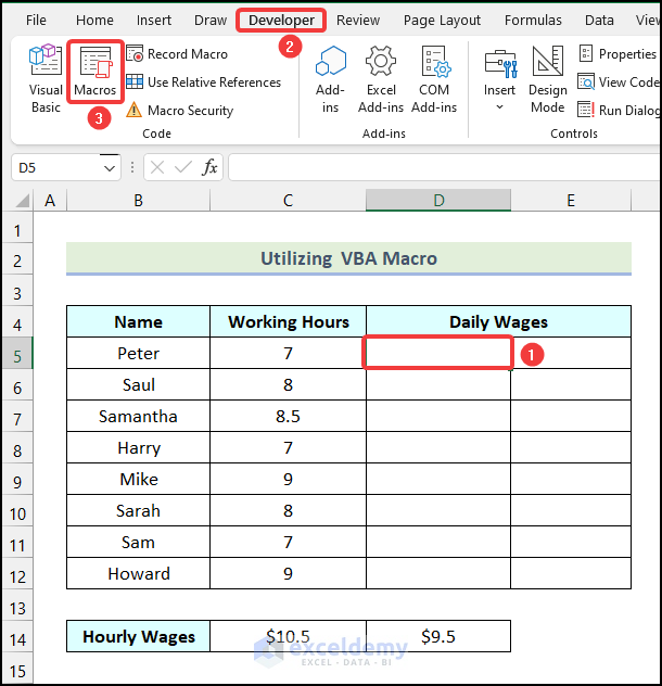
- Firstly, go to the Developer tab from Ribbon.
- After that, select the Visual Basic option from the Code group.
As a result, the Microsoft Visual Basic window will open on your worksheet.

- Now, in the Microsoft Visual Basic window, go to the Insert tab.
- Then, choose the Module option from the drop-down.

- After that, write the following code in the newly created Module.
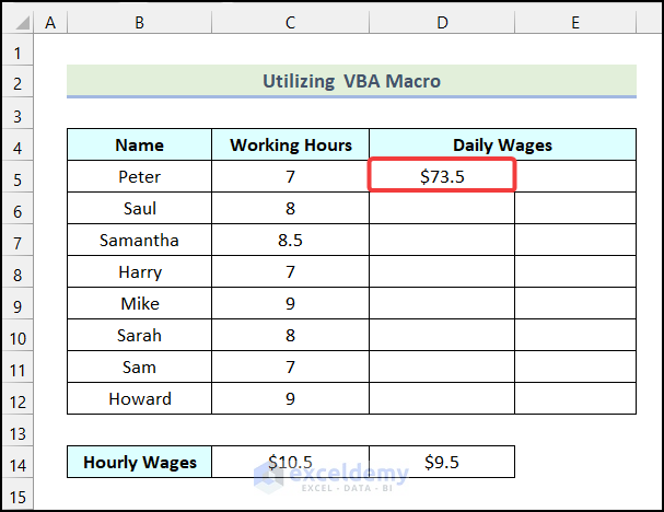
Sub FormulaRC1_Daily_Wages()
Range("D5").FormulaR1C1 = "=RC3*R14C[-1]"
End Sub
Code Breakdown
- Firstly, we initiated a sub procedure named FormulaRC1_Daily_Wages.
- Here, RC3 indicates cell C5, and R14C[-1] refers to the cell C14.
- We multiplied RC3 with R14C[-1] and assigned the value in cell D5.
- Finally, we ended the sub procedure.
- After writing the code, click on the Save option.

- Now, press the keyboard shortcut ALT + F11 to close the Microsoft Visual Basic window and open the worksheet.
- Following that, select cell D5 and go to the Developer tab from Ribbon.
- Then, click on the Macros option from the Code group.
- Afterward, from the Macro dialogue box, choose the FormulaRC1_Daily_Wages option.
- Then, click on Run.

Consequently, you will have the following output on your worksheet.
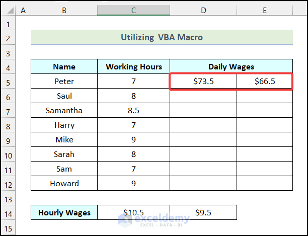
- Now, drag the Fill Handle horizontally to obtain the Daily Wages of Peter for two different Hourly Wages rates.
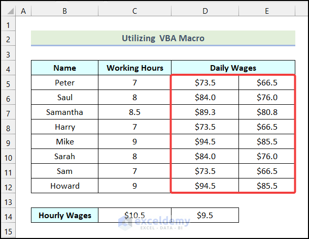
- Lastly, apply the AutoFill feature of Excel to get the remaining outputs as shown in the following picture.
How to Anchor Cells in Excel
While working in Excel, we often need to anchor cells for various calculations. For instance, we need to anchor the denominator while computing the percentages in Excel. In this section of the article, we will learn the detailed steps to anchor cells in Excel.
Steps:
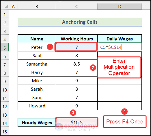
- Firstly in cell D5, type in equal (=) and select cell C5.
- Then, enter a multiplication operator (*).
- Following that, select cell C14 and press F4 once. This will anchor cell C14.
Your final formula will be like this.
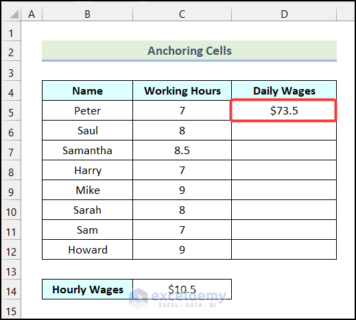
=C5*$C$14- Now, press ENTER.
Subsequently, you will have Daily Wages of Peter in cell D5.
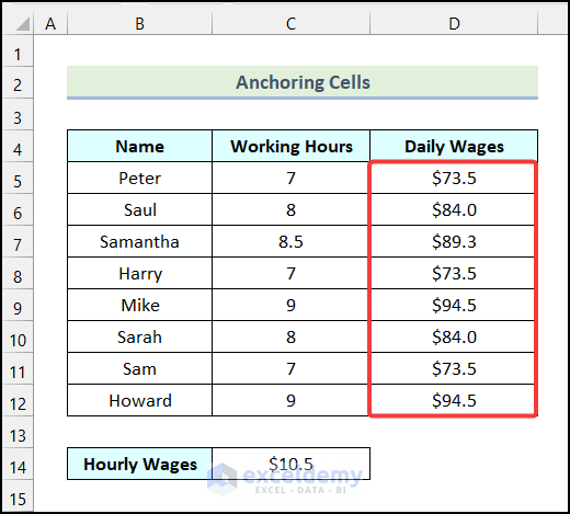
- Lastly, apply Excel’s AutoFill option to get the rest of the outputs as demonstrated in the following picture.
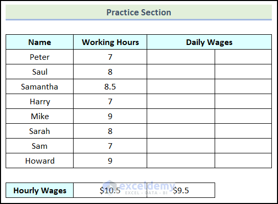
Practice Section
In the Excel Workbook, we have provided a Practice Section on the right side of the worksheet. Please practice it yourself.
Download Practice Workbook
Conclusion
So, these are the most common and effective methods you can use anytime while working with your Excel datasheet for anchoring columns in Excel. If you have any questions, suggestions, or feedback related to this article, you can comment below.
Related Articles
<< Go Back To Anchoring in Excel | Linking in Excel | Learn Excel
Get FREE Advanced Excel Exercises with Solutions!
