How to Remove Anchor in Excel (2 Easy Methods)

While working with Excel, users use various types of formulas to get desired values. In a large data set, typing the formula separately for each cell is time-consuming and tedious. Also, while dragging the formula the cell reference changes in the formula. That’s when you need to absolute the cell reference which is also known as anchoring. But, the whole absolute cell reference or anchoring is not necessary all the time. In this article, I will show you how to remove anchor in Excel.

Table of Contents hide

Download Practice Workbook

2 Easy Methods to Remove Anchor in Excel

1. Use Keyboard Shortcut

2. Run a VBA Code

Things to Remember

Conclusion

Download Practice Workbook

You can download the free Excel workbook here and practice on your own.

Removal of Anchor.xlsm

2 Easy Methods to Remove Anchor in Excel

In this article, you will see two easy methods to remove anchor in Excel. Firstly, I will use a keyboard shortcut for the removal. And secondly, I will apply a VBA code for the same.

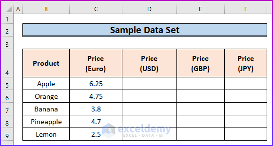
To illustrate the article further, I will use the following sample data set.

1. Use Keyboard Shortcut

The first method will include the use of a keyboard shortcut for the removal of anchoring. In this method, you will see what would happen if you use the same cell reference for the whole reference where the referenced cells are not the same for all the result cells. To learn more about this procedure, see the following steps.

Steps:

Firstly, look at the following image, where I will find out the conversion of the price in euros of each fruit in different currencies.

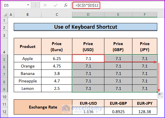
Secondly, to do that, input the following formula in cell D5.

=$C$5*$D$12

Thirdly, press Enter, and using AutoFill, you get values for the cell range D5:F9.
From the following result, you can see that the resultant prices in the cell range are all the same.
As I have anchored both the column and the row in the cell reference, it has shown the same result for the whole data range.

Fourthly, to remove the anchor from the whole cell reference and provide where only it is necessary do the following.
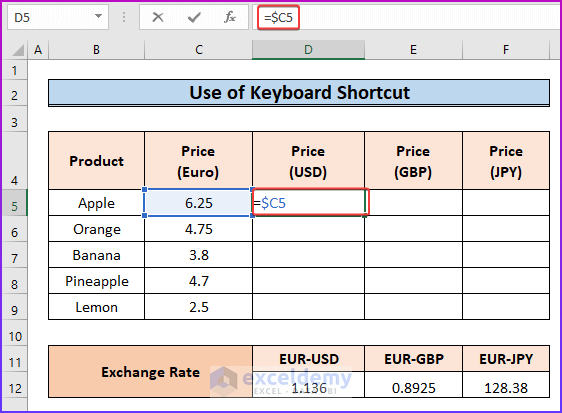
First of all, look at the previous formula, where for the cell range D5:E5, I want to show the price of apple in different currencies.
So here, I will anchor the column position of the price of apple in euros which is in column C but not the row position.
For that, after typing C5 in cell D5, press F4 on your keyboard three times, and the result will look like the following image, where I have only anchored the column.

Then, as the price of apples in different currencies are in the same row and different columns, here I want to anchor the row number only.
In order to do that, type D12 in cell D5 and again press F4 on your keyboard but this time press only twice.
By doing this, while dragging the formula only the column number will change but the row number will not.

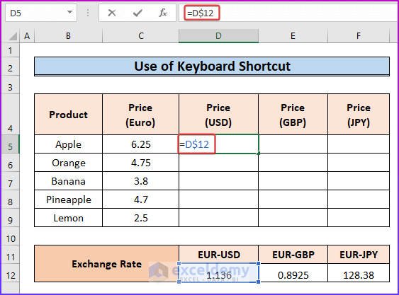
So, the whole formula after the removal of unnecessary anchoring will look like the following image.

=$C5*D$12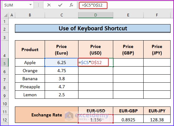

Afterward, press Enter and drag the formula using AutoFill throughout the whole resultant cell range.

Finally, you will see the desired results in all the cells, and this time the price are all accurate which were all wrong in the third step of this procedure.

Consequently, put the cursor of your mouse in any of the prices and you will see the formula without unnecessary anchoring.

2. Run a VBA Code

You will see the application of a VBA code as the second method of this procedure. By applying some commands and giving the correct sequence, you will be able to run the code and remove the unnecessary anchors. The detailed steps of this procedure are as follows.

Steps:

Firstly, from the following image, you can see the error in the price of each food in different currencies as I anchored both columns and rows in the formula.

In order to remove the anchoring with the VBA code, go to the Developer tab of the ribbon.
Then, from the Code group, select Visual Basic.

Thirdly, you will see the VBA window after the previous step.
Then, from the Insert tab select Module.

Fourthly, copy the following code and paste it into the module.

Sub Removal_of_Anchor()
Range("D5").Select
ActiveCell.FormulaR1C1 = "=RC3*R12C"
Range("D5").Select
Selection.AutoFill Destination:=Range("D5:F5"), Type:=xlFillDefault
Range("D5:F5").Select
Selection.AutoFill Destination:=Range("D5:F9"), Type:=xlFillDefault
Range("D5:F9").Select
End Sub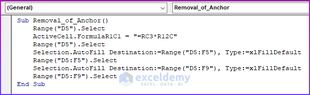

VBA Breakdown

Firstly, name the sub_procedure.

Sub Removal_of_Anchor()

Then, select the cell and insert the formula.

Range("D5").Select
ActiveCell.FormulaR1C1 = "=RC3*R12C"

Lastly, drag the formula throughout the whole resultant cell range.

Range("D5").Select
Selection.AutoFill Destination:=Range("D5:F5"), Type:=xlFillDefault
Range("D5:F5").Select
Selection.AutoFill Destination:=Range("D5:F9"), Type:=xlFillDefault
Range("D5:F9").Select

After that, save the code and press F5 or the Run button after keeping the cursor in the module.

Finally, after running the code will change the value of the D5:F9 data range.

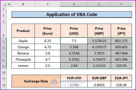
Consequently, by clicking on any of the result cells see the formula where the unnecessary anchoring is removed.

Things to Remember

While you are using any macro or VBA code, remember to enable the macro feature while saving the file.
Remember to insert proper cell references while typing the formula.

Conclusion

That’s the end of this article. I hope you find this article helpful. After reading the above description, you will be able to remove anchor in Excel. Please share any further queries or recommendations with us in the comments section below.

The ExcelDemy team is always concerned about your preferences. Therefore, after commenting, please give us some moments to solve your issues, and we will reply to your queries with the best possible solutions.