How to Add Horizontal Line in Excel Scatter Plot (2 Quick Methods)

Excel is a powerful tool to handle large data sets and charts. In Excel, we often use the Scatter Plot to visualize our data, find any correlation among the variables, and understand any trends in the data. Sometimes we need to add a horizontal line in the Excel Scatter Plot. In this article, we are going to learn 2 quick and effective methods to add horizontal line in the Excel Scatter Plot.

Download Practice Workbook

What Is a Scatter Plot?

Scatter Plots are widely used to determine any correlation among the variables of a chart. If there is any correlation, the points on the Scatter Plot will be close to each other. On the other hand, if there is no correlation then the points on Scatter Plot will be randomly distributed. By using Scatter Plot, we can also understand if there is any trend in the data set or not.

2 Methods to Add Horizontal Line in Scatter Plot in Excel

We can add horizontal lines in excel by using 2 quick methods. Now we are going to learn these 2 methods.

In the following data set, we have the Age of 10 Persons. We are going to implement a Scatter Plot using this data set and later on we will add a horizontal line to it.

1. Inserting Extra Column to Add Horizontal Line

We can add horizontal lines in a Scatter Plot very easily by adding an extra column in our data set. Let’s proceed one step at a time.

Step 1: Insert an Extra Column

Let’s assume that we are going to insert the horizontal line at Age 23. For this reason, we will create an extra column named Line Position and insert 23 in all of the cells of that column.

Step 2: Create the Scatter Plot

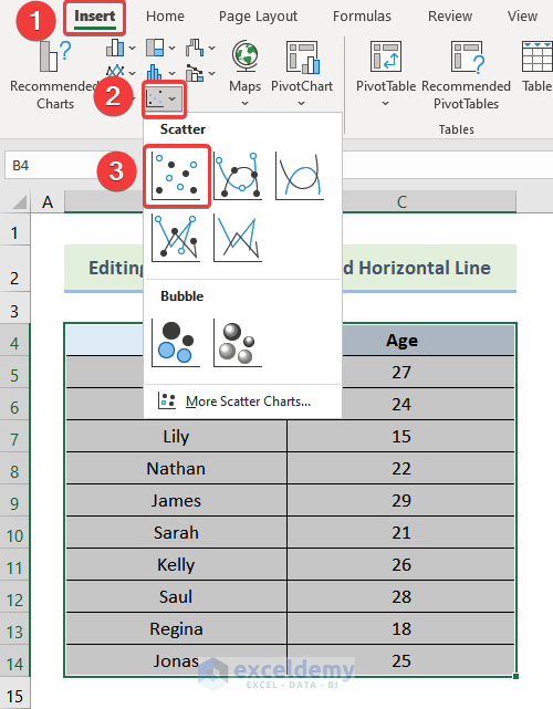
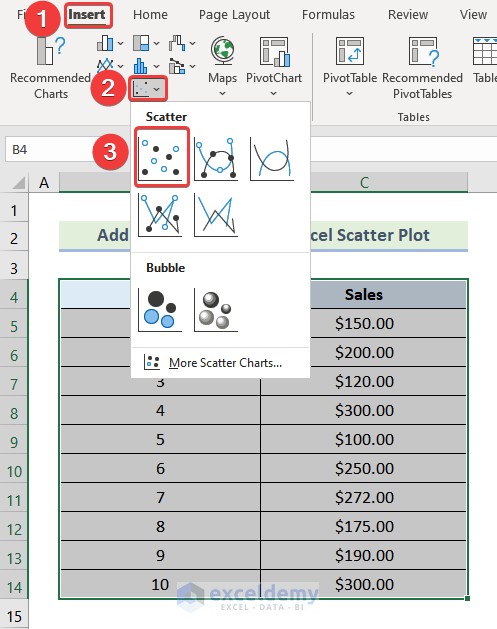
Now, select your data and go to the Insert tab from the ribbon. After that, click on Insert Scatter (X, Y) or Bubble Chart. Then select Scatter from the Scatter drop-down.

Step 3: Select Format Data Series

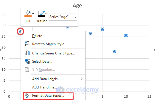
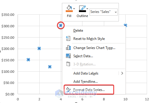
Now, right-click on any point of the series, and after that select Format Data Series.

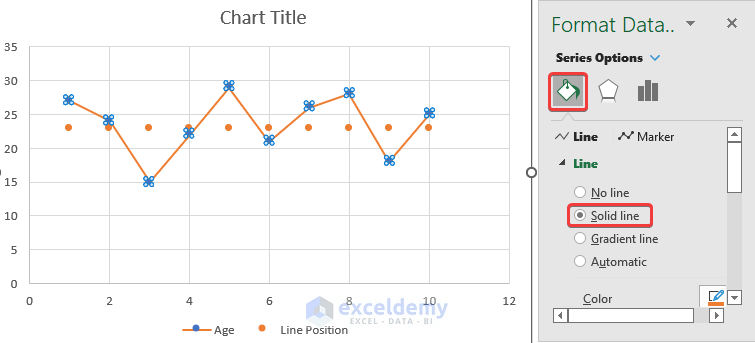
Step 4: Choose a Solid Line

Next, select Solid Line from the Format Data Series dialogue box as highlighted in the following picture.

Step 5: Click on Horizontal Line Point

Right-click on any point of the horizontal line and click on Format Data Series.

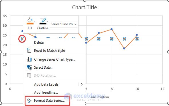
Step 6: Select Solid Line

Now, choose Solid Line from the Format Data Series dialogue box.

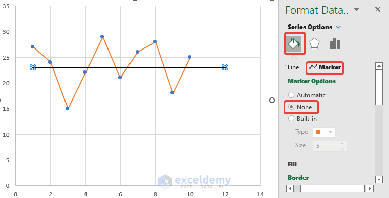
Step 7: Remove Markers of Horizontal Line

From the Format Data Series dialogue box, under the Marker tab choose None from the Marker Options.

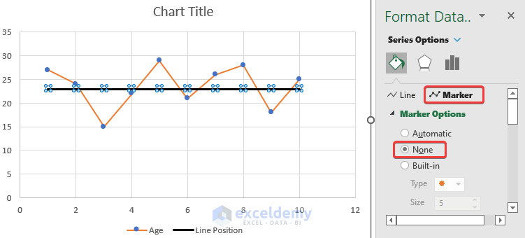
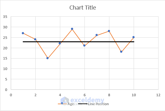
At this stage, you will be able to see the horizontal line on your Scatter Plot.

Read More: How to Add Line to Scatter Plot in Excel (3 Practical Examples)

Similar Readings

• Add Average Line to Scatter Plot in Excel (3 Ways)
• How to Connect Dots in Scatter Plot in Excel (with Easy Steps)
• Add Multiple Series Labels in Scatter Plot in Excel
• How to Combine Two Scatter Plots in Excel (Step by Step Analysis)
• Use Scatter Chart in Excel to Find Relationships between Two Data Series

2. Editing Scatter Plot to Add Horizontal Line

In this method, we are not going to use any extra column to add the horizontal line. Rather, we will edit our Scatter Plot to introduce a horizontal line in it.

Step 1: Create an Extra Column

Follow the instructions in Step 1 of the 1st Method.

Step 2: Create a Scatter Plot

Redo Step 2 of Method 1.

Step 3: Select Format Data Series

Follow the instructions in Step 3 of Method 1.

Step 4: Choose Select Data

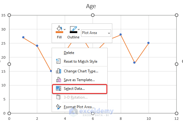
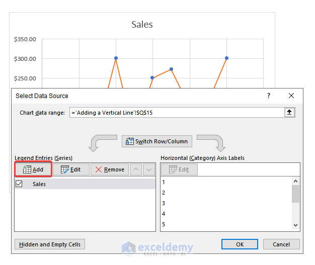
Now, right-click on any empty space in the chart and choose Select Data.

Step 5: Add New Series

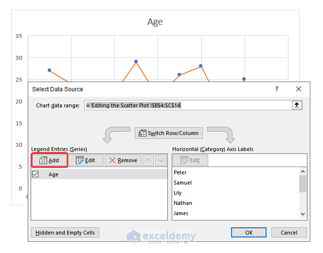
Afterward, select Add from the Select Data Source dialogue box.

Step 6: Specify the Position of the Line

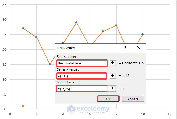
• Now another dialogue box will pop up, called Edit Series. First, name the series in the Series Name box. In this case, we are using the name, Horizontal Line.
• Then in the Series X values: box, insert the start point and end point of the X value for our horizontal line. Here it is = {1,12}.
• After that, in the Series Y values: box, enter the start point and the end point of the Y value for our horizontal line. In this case, it is = {23,23}.
• Afterward, press OK.

Step 7: Close Select Data Source Dialogue Box

Now, press OK from the Select Data Source dialogue box.

Step 8: Choose the Color of the Line

Afterward, click on the horizontal line and choose your preferred color from the Select Data Source dialogue box.

Step 9: Remove Markers of Horizontal Line

Now, use the instructions mentioned in Step 7 of Method 1.

Congratulations! You have successfully added a horizontal line to the Scatter Plot.

Read More: How to Create a Scatter Plot in Excel with 3 Variables (with Easy Steps)

How to Add a Vertical Line to a Scatter Plot in Excel

Adding a vertical line is almost similar to our 2nd Method (anchor). There is only a negligible difference while inserting data in the Edit Series dialogue box.

In the following data set, we have Sales data for 10 Days. We are going to add a vertical line in the Scatter Plot using this data set.

• Follow Step 1 of Method 1.

• Repeat the instructions mentioned in Step 2 of Method 1.

• Redo Step 3 of Method 1.

• Now, follow the instructions mentioned in Step 4 of Method 2.

• Use these instructions from Step 5 of Method 2.

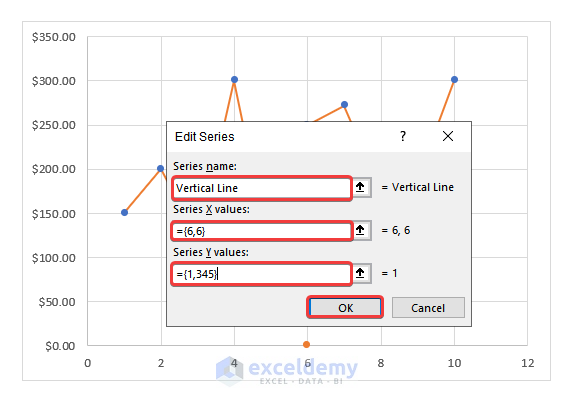
• Now, in the Edit Series dialogue box, first, insert the name of the series in the Series name box. We are using the name Vertical Line here.
• Then, insert the Series X values: box, insert the start point and end point of the X value for our horizontal line. Here it is = {6,6}.
• After that, in the Series Y values: box, insert the start point and the end point of the Y value for our horizontal line. In this case, it is = {1,345}.
• Next, press OK.

• Afterward, select OK from the Select Data Source dialogue box

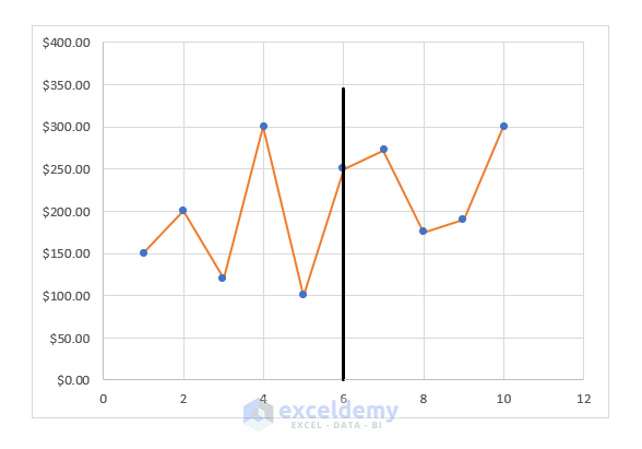
At this stage, you will be able to see the vertical line in your Scatter Plot.

Things to Remember

• While selecting data in the Method 1, you must include the extra column you added to the selection.
• In this step of Method 2, make sure that you click on the empty space on the chart.

Conclusion

Finally, we have come to the very end of the article. I sincerely hope that this article will e able to help you with adding horizontal lines to an Excel Scatter Plot. Please feel free to leave a comment if you have any queries or recommendations for improving the article’s quality. To learn more about Excel you can visit our website ExcelDemy. Happy learning!

Related Articles

• How to Make a Scatter Plot in Excel with Multiple Data Sets
• Create Excel Scatter Plot Color by Group (3 Suitable Ways)
• How to Create a Scatter Plot with 4 variables in Excel (with Quick Steps)
• Create a Scatter Plot in Excel with 2 Variables
• How to Make a Scatter Plot in Excel with Two Sets of Data (in Easy Steps)
• Add Text to Scatter Plot in Excel (2 Easy Ways)
• How to Add Data Labels to Scatter Plot in Excel (2 Easy Ways)