How to Add Gridlines in Excel After Highlighting (3 Easy Methods)

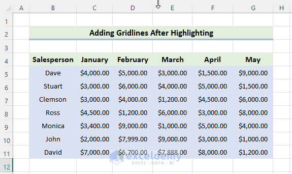
Excel worksheets and workbooks display gridlines by default. But, the gridlines disappear as soon as we highlight the cells. And many times, this is not desired. If you are looking for special tricks to add gridlines after highlighting in Excel, you’ve come to the right place. There are three suitable examples to add gridlines after highlighting in Excel. This article will discuss every step of these methods to add gridlines in Excel after highlighting. Let’s follow the complete guide to learn all of this.

How to Add Gridlines in Excel After Highlighting (3 Easy Methods)

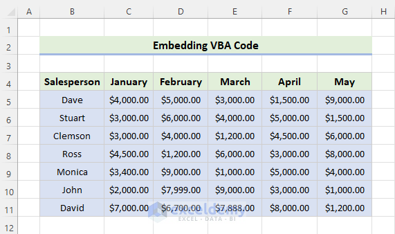
In the following section, we will use three effective and tricky methods to add gridlines after highlighting in Excel. Here, we will use three methods: using borders, use of format cells, and embedding VBA code. This section provides extensive details on these methods. You should learn and apply these to improve your thinking capability and Excel knowledge. We use the Microsoft Office 365 version here, but you can utilize any other version according to your preference. In this article, we demonstrate the above-mentioned three methods for the following dataset.

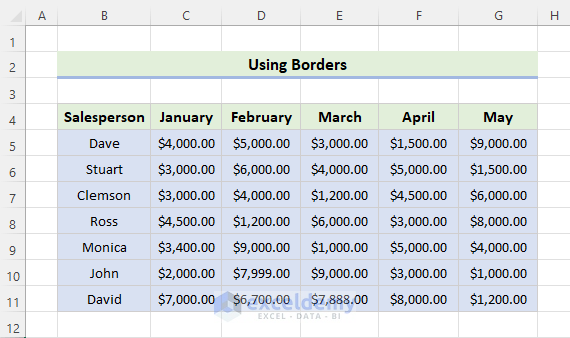
1. Using Borders

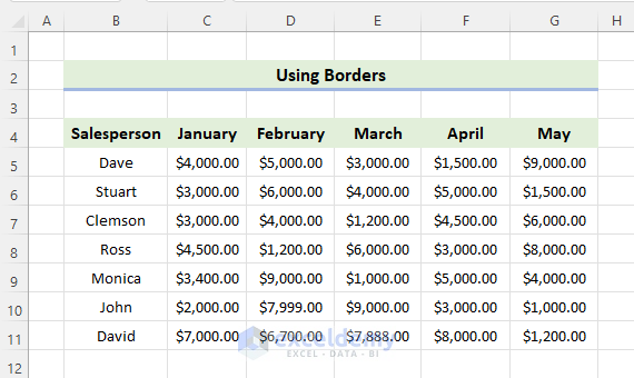
Here, we will demonstrate how to add gridlines in Excel after highlighting. Let us first introduce you to our Excel worksheet so that you are able to understand what we are trying to accomplish with this article. In the following dataset, we can see the different salesperson monthly sales. Now, we will highlight the dataset with the Fill Color option. The grid lines do not appear when we highlight the dataset. Let’s walk through the following steps to add gridlines after highlighting them in Excel.

📌 Steps:

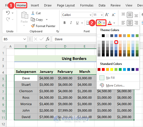
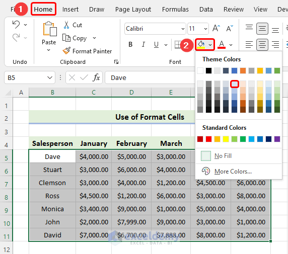
• First of all, we will highlight the dataset. To do this, select the range of the cells and go to the Home tab.
• Then, select Fill Color and choose your desired color based on your preference.

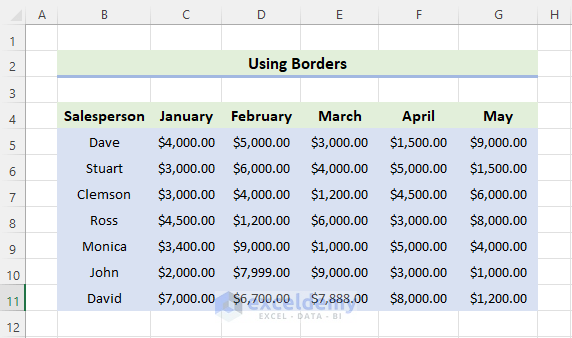
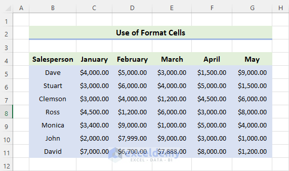
• Consequently, the dataset will look like this.

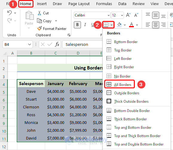
• Next, select the range of the cells, go to the Home tab, and select Borders.
• Then, from the drop-down menu select All Borders.

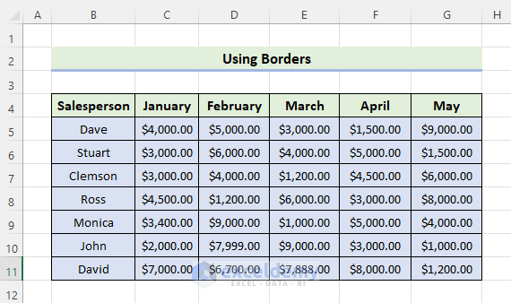
• Consequently, the dataset will look like this.

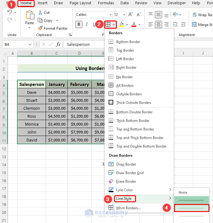
• Next, select the range of the cells and go to the Home tab.
• From the drop-down menu select Line Style and choose the dotted line as shown below.

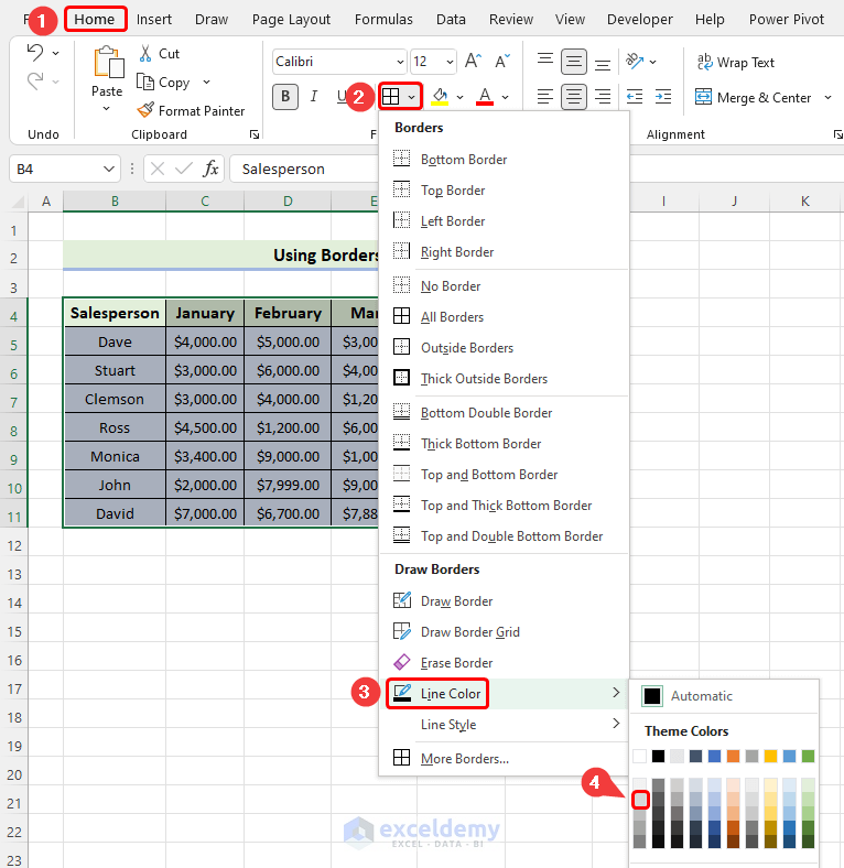
• Next, select the range of the cells and go to the Home tab.
• From the drop-down menu select Line Color and choose the color as shown below.

• As a consequence, you will be able to add gridlines in Excel after highlighting as shown below.

Read More: How to Add Gridlines for Specific Cells in Excel

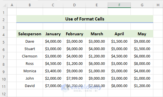
2. Use of Format Cells

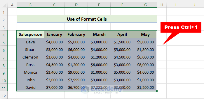
Here, we will illustrate another effective and tricky method to add gridlines in Excel after highlighting. In the following dataset, we can see the different salesperson monthly sales. Our first step will be to highlight the dataset with the Fill Color option. When we highlight the dataset, the grid lines are not visible. Let’s walk through the following steps to add gridlines after highlighting them in Excel.

📌 Steps:

• First of all, we will highlight the dataset. To do this, select the range of the cells and go to the Home tab.
• Then, select Fill Color and choose your desired color based on your preference.

• Consequently, the dataset will look like this.

• Next, select the range of the cells as shown below and press ‘Ctrl+1’ from the keyboard.

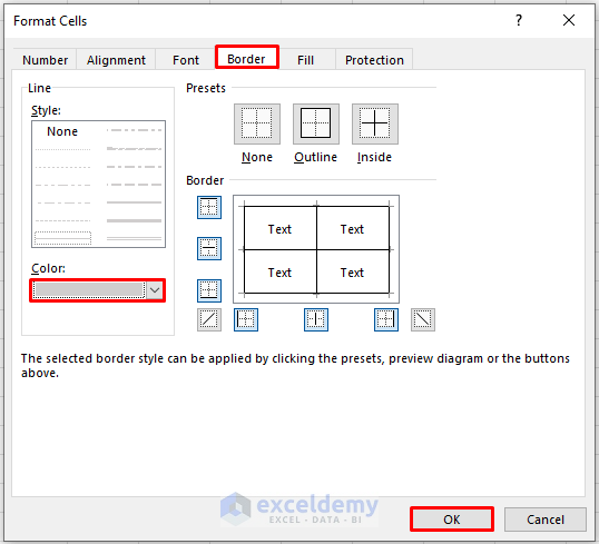
• Consequently, the Format Cells window will appear.
• Afterward, under the Border tab, select the Gray color from the Color. Here, we select Gray to match the color of the Gridlines.
• Next, click on OK.

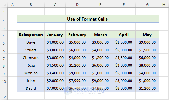
• As a consequence, you will be able to add gridlines in Excel after highlighting as shown below.

Read More: How to Add More Gridlines in Excel

3. Embedding VBA Code

If you want to add gridlines in Excel after highlighting, you need to use the help of VBA. Microsoft Visual Basic for Applications (VBA) is Microsoft’s Event Driven Programming Language. To use this feature you first need to have the Developer tab showing on your ribbon. Click here to see how you can show the Developer tab on your ribbon. Once you have that, follow these detailed steps to add gridlines in Excel.

📌 Steps:

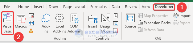
• VBA has its own separate window to work with. You have to insert the code in this window too. To open the VBA window, go to the Developer tab on your ribbon. Then select Visual Basic from the Code group.

• VBA modules hold the code in the Visual Basic Editor. It has a .bcf file extension. We can create or edit one easily through the VBA editor window. Then, click on the ThisWorkbook.

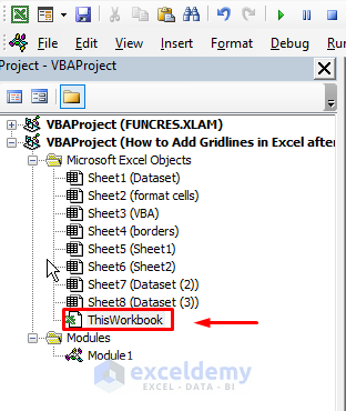
• As a result, a dialog box will emerge.
•  Then write down the following code in it.

Dim rng As Range
Private Sub Workbook_SheetSelectionChange(ByVal Sh As Object, ByVal Target As Range)
    On Error Resume Next
    If Not rng Is Nothing Then Insert_Borders rng
    Set rng = Target
End Sub
Private Sub Insert_Borders(ByVal rg As Range)
    Dim cells As Range
    Application.ScreenUpdating = False
    For Each cells In rg
        If cells.Interior.ColorIndex = xlNone Then
            With cells.Borders
                If .ColorIndex = 15 Then
                    .LineStyle = xlNone
                End If
            End With
        Else
            With cells.Borders
                If .LineStyle = xlNone Then
                    .Weight = xlThin
                    .ColorIndex = 15
                End If
            End With
        End If
    Next
    Application.ScreenUpdating = True
End Sub

Next, save the code and close the VBA window.

• Lastly, highlight the range B4:G11 in Blue color and the gridlines will appear automatically.

Download Practice Workbook

Download this practice workbook to exercise while you are reading this article. It contains all the datasets in different spreadsheets for a clear understanding. Try yourself while you go through the step-by-step process.

Conclusion

That’s the end of today’s session. I strongly believe that from now you may be able to add gridlines in Excel after highlighting. If you have any queries or recommendations, please share them in the comments section below.