To change date format using a formula in Excel, apply the following steps:
- Select a cell.
- Insert the formula: =TEXT(Reference Cell,”Date Format”)
- Press Enter.
For example, to change the format to dd-mm-yyyy for a date in cell A1, you can apply the formula: =TEXT(A1,”dd-mm-yyyy”)
Different regions and users prefer distinct date formats. By adjusting the date format, you ensure that the data is easily understood and aligned with local conventions. Excel provides options for changing the date format according to your needs.
In this Excel tutorial, you will learn how to change date format using a formula in Excel.
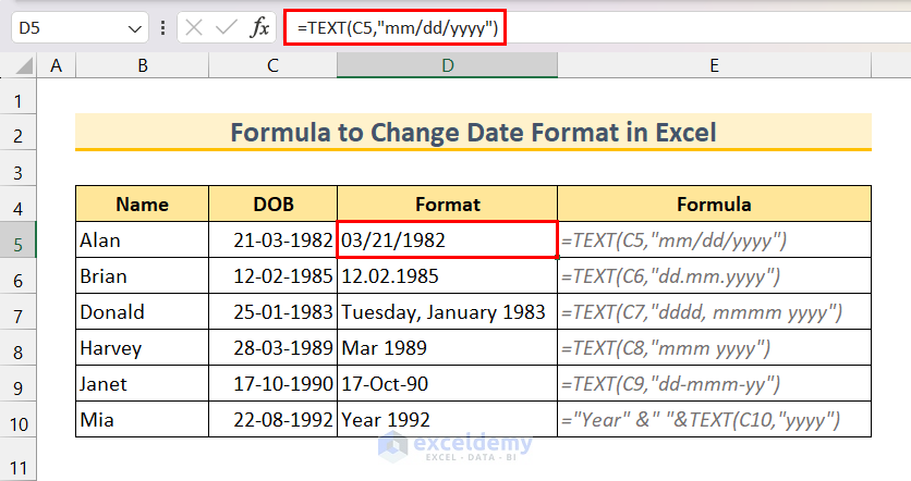
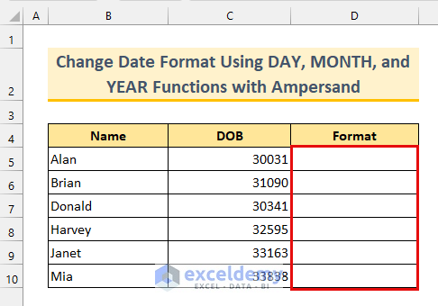
Consider a dataset with a list of dates of births. I have changed the format of the dates using a formula.
How to Use Date Format in Excel?
A date format in Excel refers to how dates are displayed in a cell. Excel stores dates as serial numbers, starting from January 1, 1900, as 1. Each day that follows is represented by a whole number increment. For example, January 2, 1900, is 2, and so on.
By using Excel’s predefined or custom date formatting, you can display the serial numbers in a readable date format. This formatting doesn’t change the underlying serial number value.
Here is a list of common predefined date formats in Excel:
| Date Format | Description | Example (8th January, 2024) |
|---|---|---|
| mm/dd/yyyy | Month-Day-Year format | 01/08/2024 |
| dd/mm/yyyy | Day-Month-Year format | 08/01/2024 |
| dd-m-yy | Day-Month (1 digit)-Year (2 digit) format | 08-1-24 |
| dd-mmm-yy | Day-Month abbreviation-Year format | 02-Jan-2024 |
| dddd, mmmm d, yyyy | Full weekday name, full month name, day, year format | Monday, January 8, 2024 |
If you require a date format other than the predefined date formats, you can create a custom date format. To create a custom date format, you can use the following codes:
| Code | Description | Example (8th January, 2024) |
|---|---|---|
| d | day number of the mon without a leading zero | 8 |
| dd | day number of the month with a leading zero for single-digit days | 08 |
| ddd | abbreviated day of the week | Mon |
| dddd | full day of the week | Monday |
| m | month number as a single digit without a leading zero | 1 |
| mm | month number as a two-digit number with a leading zero for single-digit months | 01 |
| mmm | abbreviated month name | Jan |
| mmmm | full month name | January |
| yy | last two digits of the year | 24 |
| yyyy | four-digit year | 2024 |
Using the above codes and a suitable separator such as Slash (/), Hyphen (-), Period (.), Comma (,), and Space ( ) you can create a custom date format.
5 Formulas to Change Date Format in Excel
For changing a date format with a formula, we usually use the TEXT function. If dates are stored as numbers or text, then you can use LEFT, MID, and RIGHT functions to extract the year, month, and day parts of a date and then create a proper date format using the DATE function.
And, if you want to change the date separator, then you can extract year, month, and day parts using the YEAR, MONTH, and DAY functions respectively, and then format with the desired date separator by using the SUBSTITUTE or CONCATENATE function.
Here are 5 formula examples to change a date format in Excel:
Using the TEXT Function
The TEXT function is useful for changing the way a number appears by applying desired formatting to it with format codes. You can use this function to change a date format to your desired date format.
To change a date format using the TEXT function, follow the steps below:
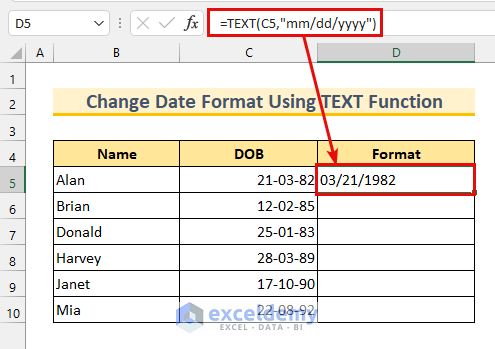
- Select an empty cell.
- Apply the formula:
=TEXT(C5,"mm/dd/yyyy")
Here, C5 refers to the date for which you want to change the format, and mm/dd/yyyy is the date format you want to apply. Replace these arguments with target cell reference and desired format. - Press Enter.
The date format has now changed.
- Repeat the above steps for other cells.
Here we have shown formulas for the remaining cells with various date formats.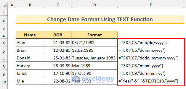
Read More: How to Convert Date to Text YYYYMMDD
Combining DATE, LEFT, RIGHT, & MID Functions
Sometimes dates can be formatted with other number formats such as Number or Text. To change the date format with a formula, we can combine the DATE, LEFT, MID, and RIGHT functions.
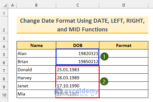
Consider a dataset where some dates are in number format (right alignment) and some other dates are in text format (left alignment).
Here are two cases to change the date format with a formula combining DATE, LEFT, MID, and RIGHT functions:
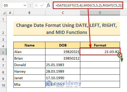
Case 1: Dates Are in Number Format
In our number formatted date, the left 4 digits refer to the year value, the mid 2 digits starting from the 5th digit refer to the month value, and the right 2 digits depict the day values.
To change date format with a formula in such case, you can apply the following steps:
- Select a cell.
- Insert the formula:
=DATE(LEFT(C5,4),MID(C5,5,2),RIGHT(C5,2))
Replace C5 with the cell that contains the date you want to format. - Press Enter.
Case 2: Dates Are in Text Format
In our dataset, the right 4 digits depict the year value, the mid 2 digits starting from the 4th digit refer to the month value, and the left 2 digits depict the day value.
To apply a formula to change the date format in such case, you can apply the following steps:
- Select a cell.
- Insert the following formula:
=DATE(RIGHT(C7,4),MID(C7,4,2),LEFT(C7,2))
Here, replace C5 with the cell that contains the date you want to format. - Press Enter.
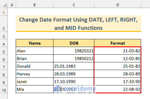
- Drag the Fill Handle icon down to copy the formula in the remaining cells.
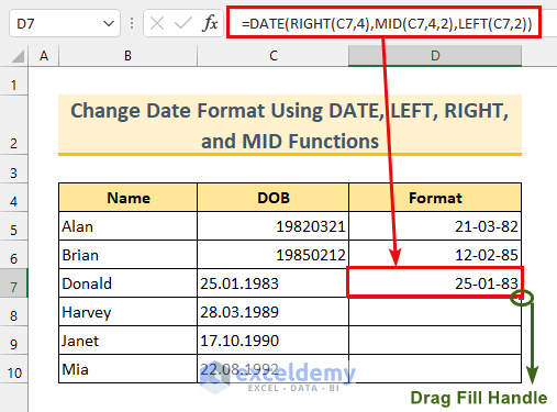
As a result, the text-formatted dates will change to the proper date format.
Read More: How to Convert Date to Text Month in Excel
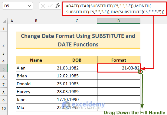
Using SUBSTITUTE, DATE, YEAR, MONTH, & DAY Functions
Consider the following where dates are formatted as text (left-aligned). As a date-separator, we have used period (.) here. If you want to separate year, month, and day values from such text-formatted dates using YEAR, MONTH, and DAY functions in this case, you will get #VALUE! errors.
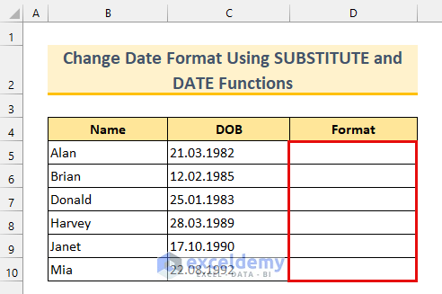
To change the date format here, you first have to replace each period (.) with the SUBSTITUTE function and then apply date formatting.
Apply the following steps to change date formatting here:
- Select a cell.
- Apply the following formula:
=DATE(YEAR(SUBSTITUTE(C5,".","-")),MONTH(SUBSTITUTE(C5,".","-")),DAY(SUBSTITUTE(C5,".","-")))
Here, C5 refers to the cell that contains a text-formatted date with a period (.) separator. - Press Enter.
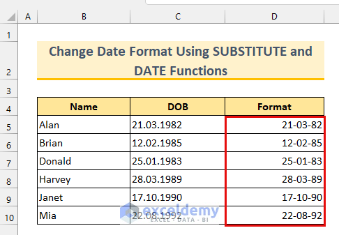
- Finally, apply the formula to other cells using the Fill Handle tool.
Thus the text-formatted dates in Excel will change to proper date format. You will also notice that the output dates are right-aligned just like properly formatted dates.
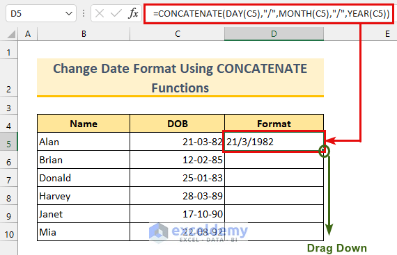
Applying CONCATENATE, DAY, MONTH, & YEAR Functions
If you wish to change the date separator or change the sequence year, month, and day values you can the CONCATENATE function to change the date format. However, the output date will be in text format in this case.
Here, I will change the date separator from hyphen (-) to slash (/). Apply the steps below:
- Select a cell.
- Apply the following formula:
=CONCATENATE(DAY(C5),"/",MONTH(C5),"/",YEAR(C5)) - Press Enter.
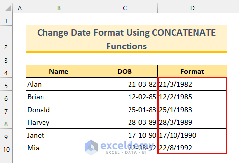
- Drag down the Fill Handle icon to copy the formula in the remaining cells.
As a result, the date separators will change in the output dates.
Read More: How to Convert Date to Julian Date in Excel
Using Ampersand Operator With MONTH, DAY, & YEAR Functions
To change any date separator or change the date format, we can use the Ampersand (&) operator as an alternative to the CONCATENATE function. However, the output date will appear in text format here as well.
To demonstrate this method, we have taken dates in serial number format. However, you can take them in any proper date format.
To change any date format with the ampersand operator formula, apply the steps below:
- Select a cell.
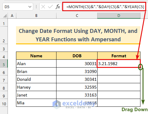
- Insert the formula:
=MONTH(C5)&"."&DAY(C5)&"."&YEAR(C5)
Here, C5 refers to the cell for which you want to change the date format and I have used period (.) as the date separator. - Press Enter.
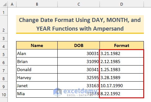
- Use the Fill Handle tool to copy the formula down.
Our goal of changing the date format using a formula is now complete.
Download Practice Workbook
Conclusion
This concludes our tutorial on how to change the date format using a formula in Excel. We discussed 5 examples that you can use to change any improperly formatted date to your desired format. If you have any queries about this article, feel free to share them in the comment section.
Frequently Asked Questions
How to format date in Excel?
You can use the Format Cells dialog box to format dates by applying a predefined or custom date format. Here’s how:
- Select the cells containing the dates that you want to format.
- Press Ctrl+1 (Cmd+1 on a Mac) to open the Format Cells dialog box.
- To select a predefined date format, go to Number > Category > Date.
To select a custom date format, go to Number > Category > Date. - Select a predefined date format or write the desired custom date format.
- Click OK.
The date format of the selected cells will change to the target date format.
How to automatically change the date in Excel?
To automatically update the date in Excel, you can use the TODAY function. Insert the following formula in the cell where you want the date:
=TODAY()
This cell will now display the current date, and it will automatically update every time you open or recalculate the spreadsheet.
What is the shortcut for converting date format in Excel?
The keyboard shortcut to convert the date format is Ctrl+Shift+3. Select the cells that you convert to date and use the keyboard shortcut Ctrl+Shift+3 to apply date format.
Note: The actual shortcut for the date format is CTRL+# but to get the # symbol you have to press SHIFT+3 so the shortcut becomes CTRL+SHIFT+3.
Related Articles
- How to Convert 7 Digit Julian Date to Calendar Date in Excel
- How to Remove Year from Date in Excel
- Stop Excel from Converting Date to Number in Formula
<< Go Back to Change Date Format | Date Format | Number Format | Learn Excel
Get FREE Advanced Excel Exercises with Solutions!

Hi,
Need Help Here Pls
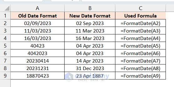
I have different date format as below in same column,
Need formula to change as DD MMM YYYY
Query Need result as
02/09/2010 02 Sep 2010
11/03/2023 11 Mar 2023
16/03/2023 16 Mar 2023
40423 04 Apr 2023
4042023 04 Apr 2023
20230404 04 Apr 2023
Thanks, LOKESH for your query. In Excel, if you want to convert different date formats into a specific date format with a single formula, the formula will be rather long and complicated. However, you can create a custom function using the following VBA code to do your task.
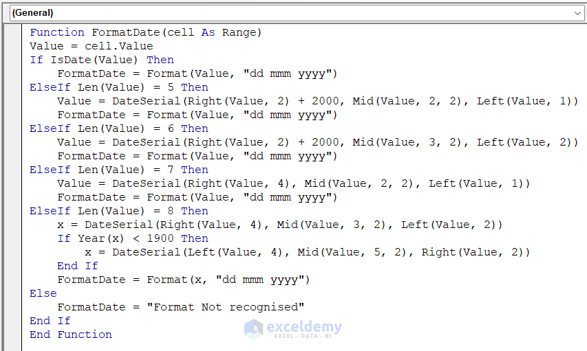
Code Syntax:
Function FormatDate(cell As Range)
Value = cell.Value
If IsDate(Value) Then
    FormatDate = Format(Value, "dd mmm yyyy")
ElseIf Len(Value) = 5 Then
    Value = DateSerial(Right(Value, 2) + 2000, Mid(Value, 2, 2), Left(Value, 1))
    FormatDate = Format(Value, "dd mmm yyyy")
ElseIf Len(Value) = 6 Then
    Value = DateSerial(Right(Value, 2) + 2000, Mid(Value, 3, 2), Left(Value, 2))
    FormatDate = Format(Value, "dd mmm yyyy")
ElseIf Len(Value) = 7 Then
    Value = DateSerial(Right(Value, 4), Mid(Value, 2, 2), Left(Value, 1))
    FormatDate = Format(Value, "dd mmm yyyy")
ElseIf Len(Value) = 8 Then
    x = DateSerial(Right(Value, 4), Mid(Value, 3, 2), Left(Value, 2))
    If Year(x) < 1900 Then
        x = DateSerial(Left(Value, 4), Mid(Value, 5, 2), Right(Value, 2))
    End If
    FormatDate = Format(x, "dd mmm yyyy")
Else
    FormatDate = "Format Not recognised"
End If
End Function
Here, I have created a Custom Function named FormatDate. Then, I apply the function to different date formats that you provided. Here is the result.
Hopefully, it will solve your problem. If you face problems anymore, feel free to post them on our Exceldemy Forum.
Regards
Aniruddah