Nested ANOVA in Excel (Detailed Analysis with Examples)

Analysis of Variance or ANOVA is a useful analysis. From the very beginning of the development of the process in 1918, it has been used widely. It shows the statistical difference between mean and different groups and determines how much each of their values correlates. A nested ANOVA is where these groups are subdivided into many groups that we may or may not correlate to individually. This article will discuss the overview of nested ANOVA and how to perform the analysis in Excel.

What Is ANOVA Anlaysis?

ANOVA is a statistical method used to analyze variance observed within a dataset. To perform it, we need to divide the dataset into two sections- systematic and random factors.

ANOVA lets us determine which factors significantly impact a given set of data. After completing the analysis, an analyst usually performs extra analysis on the methodological factors that significantly impact the inconsistent nature of data sets. In that case, he needs to use the ANOVA findings to create extra data relevant to the estimated regression analysis. The ANOVA compares many data sets to see whether there is a link between them.

There are two types of ANOVA, one is a single factor and another is two factors. In a single factor, ANOVA finds the effect of one factor on a single variable. On the other hand, there are multiple dependent variables in two factors ANOVA.

Overview of Nested ANOVA

A Nested ANOVA, as the name suggests, contains at least one factor nested inside another.

Let’s say there are two stores of a specific organization at two different places. For example, there are 2 teams- teams A and B in the first store and teams C and D in the second. Their sells assigned within their respective team would be nested within the store.

Figuratively, It will be like this.

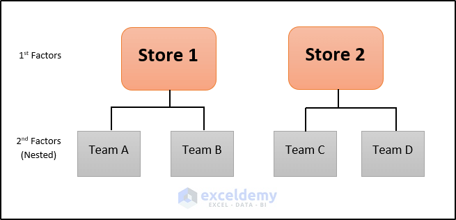
As you can see from the figure, the second factor is nested inside the first factor. Hence, ANOVA analysis of such sales would be in the nested ANOVA category.

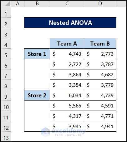
Now the data from the readings or data entries will look like this on the spreadsheet.

From this data, we can analyze two things- are the sales equal across each store (factor 1) and each team (factor 2)?

Upon performing ANOVA on this data (more of it in the later section), we will find something like this.

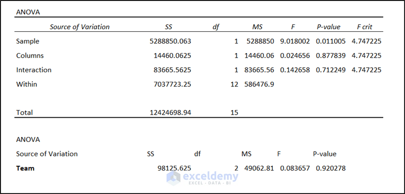
The p-values here will judge the significance of each factor. From this data, we can see that the store has a statistically significant effect whilst teams in them do not.

More of these calculations and interpretations are in the next section.

How to Perform Nested ANOVA in Excel

There is no direct way to perform a nested ANOVA in Excel. However we can still perform the operation by modifying the dataset and doing some manual calculations. We will utilize the Data Analysis Toolpak’s Two Factor with Replication feature here. Keep in mind, you may not have the Data Analysis Toolpak by default in your ribbon. In that case, you will need to enable Data Analysis Toolpak. In the end, we are gonna need the F.DIST.RT function for the manual calculation.

But first, we need to modify the original raw dataset. Because we will be performing the two factor with replication on it. Let’s take the raw dataset from the previous section.

Now follow these steps to see the steps to perform the nested ANOVA in Excel.

Steps:

First, rearrange the dataset into the following. We included teams C and D’s sales values under A and B so that Excel can read them.

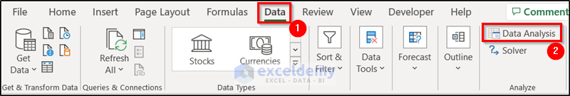
Now go to the Data tab on your ribbon.
Then select Data Analysis from the Analyze group section.

the Data Analysis box will appear.
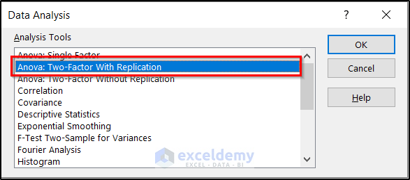
Now select Anova: Two-Factor with Replication under the Analysis Tools
Then click on OK.

Next, Anova:Two-Factor With Replication box will appear. Select the following particulars in the box.
First, enter the range B4:D12 as the input range.
Second, insert 4 in the Rows per sample field, as we have four entries for each of the nested factors.
You can change the Alpha value too if you like. But we will keep it at 0.05 for now.
Third, you can select where you want your results to display under the Output options.

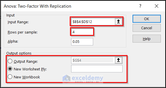
When you are done with all of these, click on OK.
As a result, the result will pop up at the location you selected. We will use the last portion under ANOVA for the nested ANOVA analysis in Excel.

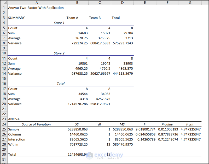
The p-value of the sample in cell F25 indicates the significance of the sample which is, in this case, the first factor, store.
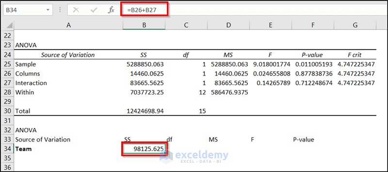
For the significance of other factors, we now need to perform some manual calculations.
First of all, select cell B34 and write down the following formula.

=B26+B27

Then press Enter.

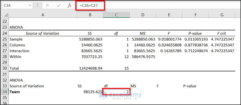
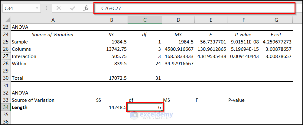
Now enter the following formula in cell C34 and press Enter.

=C26+C27

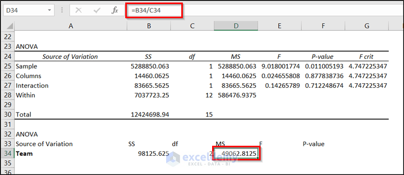
Next, insert the following formula in cell D34 and press Enter.

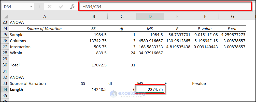
=B34/C34

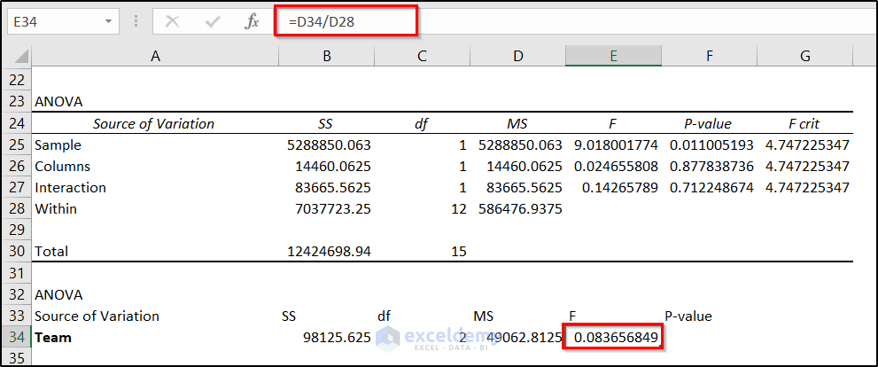
After that, use the following formula in cell E34.

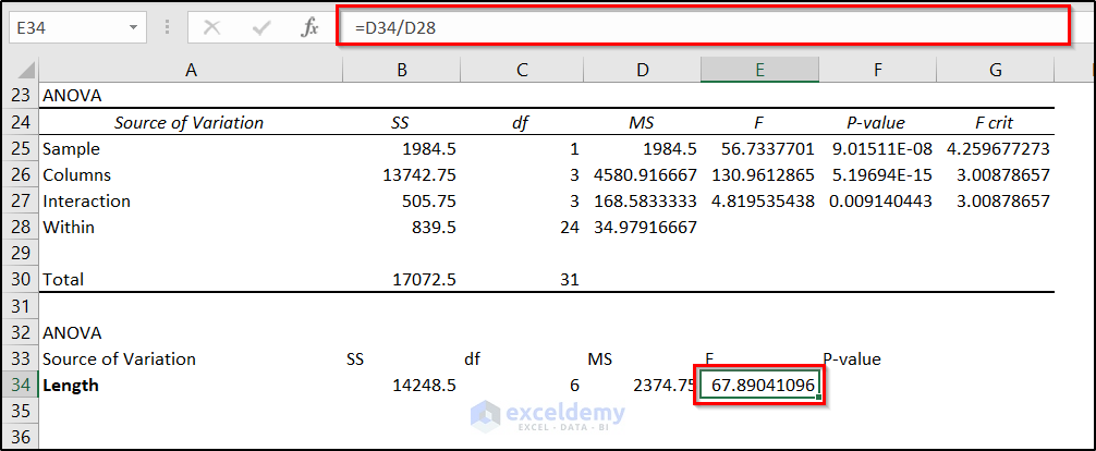
=D34/D28

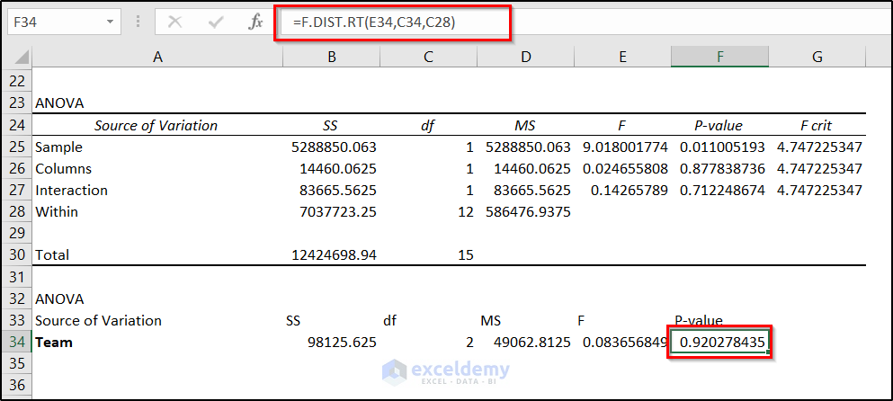
Finally, use the following formula in cell F34 and then press Enter.

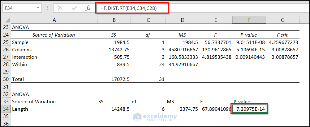
=F.DIST.RT(E34,C34,C28)

Interpretation of the Result

If a p-value of a factor from an ANOVA analysis yields a value less than 0.05 it has a significant effect on the data. In this example, we had two factors- stores and teams, where teams were nested inside the store. The p-value of the store for this data is in cell F25 and the p-value of teams is in cell F34.

As you can see from the result the p-value of the store is 0.011005 which is lower than 0.05. This indicates a significant effect on sales of this factor. Whilst p-value of the factor team is 0.9202 which is higher than 0.05. Which doesn’t indicate a significant effect on the data or sales. So we can safely conclude that the store location is more important than the combination of employees for teams in this case.

This is how we can perform a nested ANOVA in Excel.

Nested ANOVA in Excel: 2 Suitable Examples

The general idea of performing the nested ANOVA is the same in Excel. Now we will apply the same in two different examples to demonstrate its usage in different cases. Keep in mind that, we need the Data Analysis Toolpak available in the ribbon. If you don’t have one, you will need to enable Data Analysis Toolpak.

1. Calculating Variance of Resistance with Different Lengths

In this first example, we will use the following dataset.

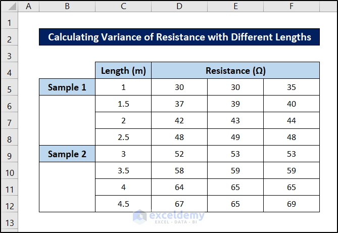
You can say there are two nests here- resistance values are nested inside length, which in turn is nested inside different samples.

But the basic idea is to use the two-factor with replication for the dataset. So we need the dataset in this way. And just like before, we are gonna need the F.DIST.RT function for the manual calculation in the end. Follow the steps to see how we can perform ANOVA in this nested dataset in Excel.

Steps:

First, go to the Data tab on your ribbon.
Then select Data Analysis from the Analyze group section.

the Data Analysis box will appear.
Now select Anova: Two-Factor with Replication under the Analysis Tools
Then click on OK.

Next, Anova:Two-Factor With Replication box will appear. Select the following particulars in the box.
First, enter the range B4:F12 as the input range.
Second, insert 4 in the Rows per sample field, as we have four entries for each of the nested factors.
You can change the Alpha value too if you like. But we will keep it at 05 for now.
Third, you can select where you want your results to display under the Output options.

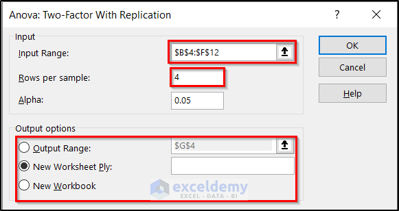
When you are done with all of these, click on OK.
As a result, the result will pop up at the location you selected. We will use the last portion under ANOVA for the nested ANOVA analysis in Excel.

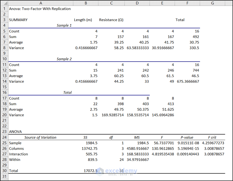
The p-value of the sample in cell F25 indicates the significance of the sample which is, in this case, the first factor, sample.
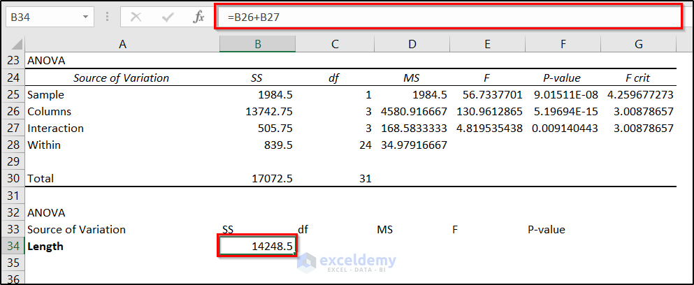
Now select cell B34 and write down the following formula.

=B26+B27

Then press Enter.

Now enter the following formula in cell C34 and press Enter.

=C26+C27

Next, insert the following formula in cell D34 and press Enter.

=B34/C34

After that, use the following formula in cell E34.

=D34/D28

Finally, use the following formula in cell F34 and then press Enter.

=F.DIST.RT(E34,C34,C28)

Interpretation of the Result

In the final result, the p-value in cell F25 indicates the significance of the sample (of different lengths) and the value of cell F34 indicates the significance of length on resistance. As both of them are below the alpha value of 0.05, they both are significant factors in this example.

2. Analyzing Variance of Marks from Different Sections

In this second example, we will use the following dataset.

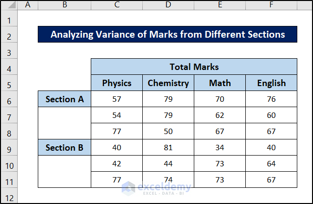
Again, this may look like a dataset for a two-way ANOVA. But this is a rearranged nested ANOVA for performing analysis in Excel. And just like before, we are gonna need the F.DIST.RT function for the manual calculation in the end.

Follow these steps to see how you can perform this nested ANOVA in Excel.

Steps:

First, go to the Data tab on your ribbon.
Then select Data Analysis from the Analyze group section.

the Data Analysis box will appear.
Now select Anova: Two-Factor with Replication under the Analysis Tools
Then click on OK.

Next, Anova:Two-Factor With Replication box will appear. Select the following particulars in the box.
First, enter the range B5:F11 as the input range.
Second, insert 3 in the Rows per sample field, as we have three entries for each of the nested factors.
You can change the Alpha value too if you like. But we will keep it at 05 for now.
Third, you can select where you want your results to display under the Output options.

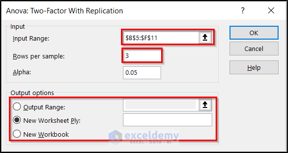
When you are done with all of these, click on OK.
As a result, the result will pop up at the location you selected. We will use the last portion under ANOVA for the nested ANOVA analysis in Excel.

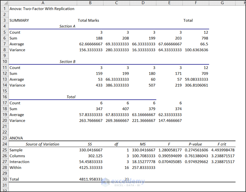
The p-value of the sample in cell F25 indicates the significance of the sample which is, in this case, the first factor, section.
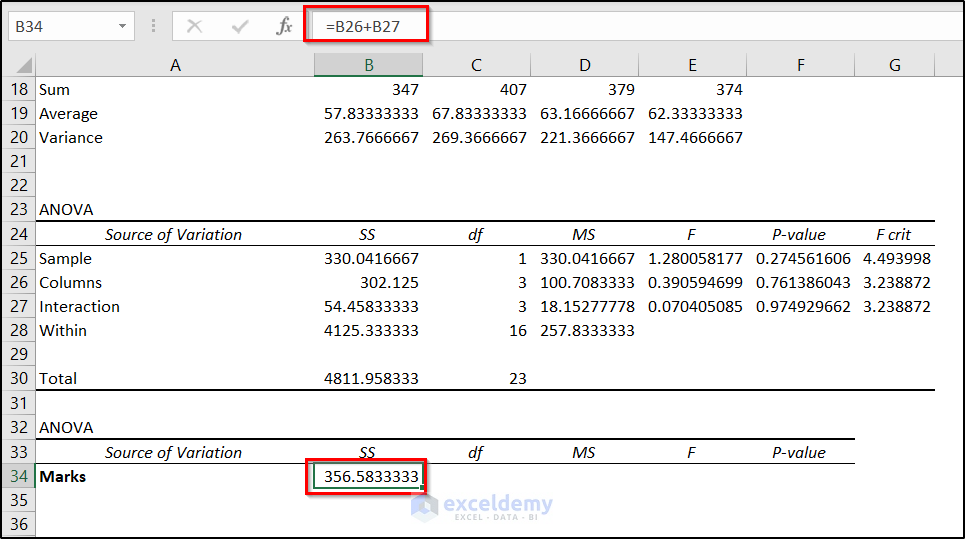
Now select cell B34 and write down the following formula.

=B26+B27

Then press Enter.

Now enter the following formula in cell C34 and press Enter.

=C26+C27

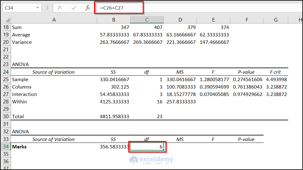
Next, insert the following formula in cell D34 and press Enter.

=B34/C34

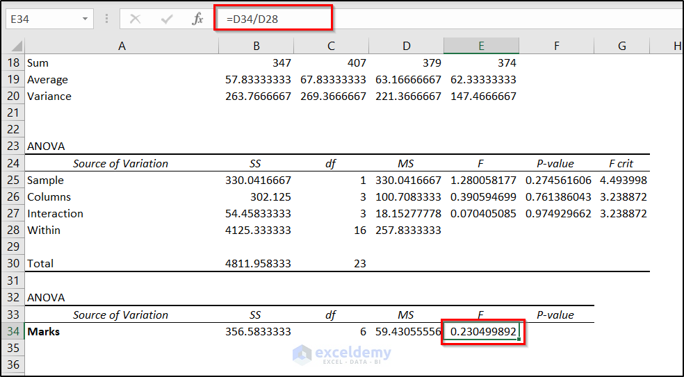
After that, use the following formula in cell E34.

=D34/D28

Finally, use the following formula in cell F34 and then press Enter.

=F.DIST.RT(E34,C34,C28)

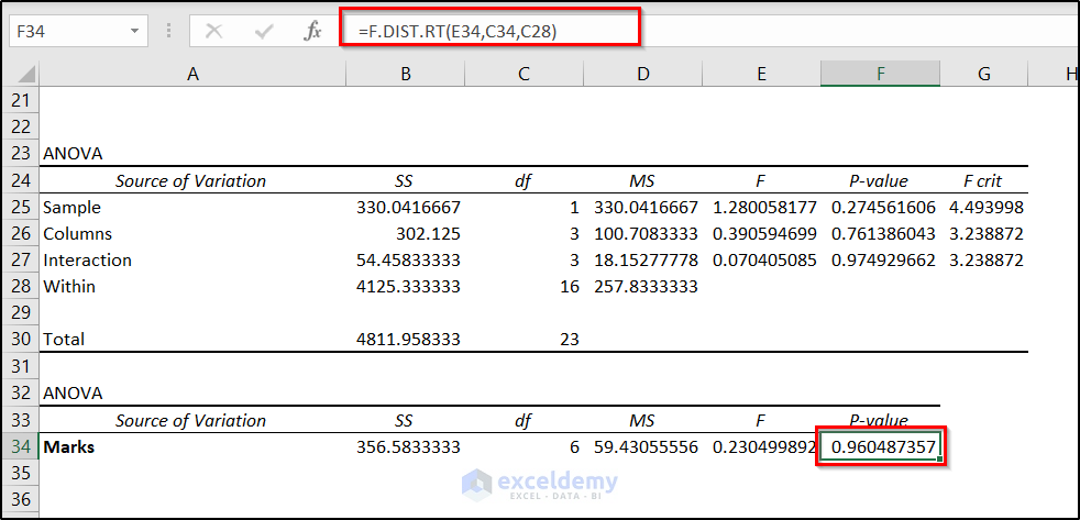
Interpretation of the Result

The p-value in cell F25 indicates the significance of the section on the statistics. This value is greater than the alpha value of 0.05. So this doesn’t have much significance. The cell value of F34 is the p-value of subject marks in the dataset. This, too, is higher than 0.05. So, again, this doesn’t have any significant effect on the marks on different subjects in different sections too for this dataset.

This is another example of how we can perform nested ANOVA in Excel.

Things You Should Remember About Nested ANOVA

A nested ANOVA can have more than two factors. Like the one used in the first example of the previous section, a factor can be nested into one factor. That factor can also be nested into another one on the hierarchy along with other factors of the same level.
A nested ANOVA is different than a two-way ANOVA. A two-factor ANOVA consists of two factors. Meanwhile, a nested ANOVA must have one of those factors nested inside the other. Which isn’t the case for the two-way ANOVA.

Download Practice Workbook

You can download the workbook used for the demonstration from the link below.

Nested ANOVA.xlsx

Conclusion

So this was the method to perform a nested ANOVA in Excel. Hopefully, you have grasped the concept of using nested ANOVA in Excel with the two-way replication feature and can use it accordingly for your datasets. I hope you found this guide helpful and informative. If you have any questions or suggestions, let us know in the comments below.

<< Go Back to Anova in Excel | Excel for Statistics | Learn Excel

Get FREE Advanced Excel Exercises with Solutions!