Average letter grades are popularly used in educational institutions to represent the results. We can easily perform this using MS Excel. There are several ways to do this in Excel. In this article, we will explain 4 of those methods to average letter grades in Excel with proper illustrations.
Download Practice Workbook
Download this practice workbook to exercise while you are reading this article.
4 Formulas to Average Letter Grades in Excel
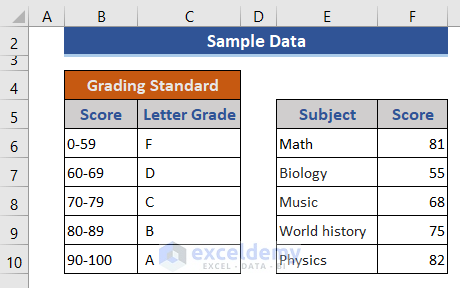
Educational institutions have their standard to calculate the average letter grades. A sample letter grade standard is shown in the dataset below to calculate the average letter grade.
1. Use IF and AVERAGE Functions to Calculate Average Letter Grades
In this section, we will first find out the average of the score using the AVERAGE function. Then, we will use the IF function to get the letter grade.
The IF function checks whether a condition is met and, returns one value if True and another if False.
The AVERAGE function returns the average (arithmetic mean) of its arguments, which can be numbers or names, arrays or references that contain numbers.
📌 Steps:
- First, we add two new rows to the sheet.
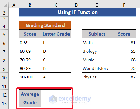
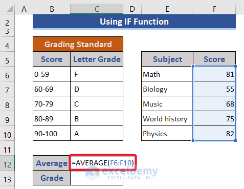
- Now, we will calculate the average score in Cell C12.
- For that, go to that cell and put the following formula.
=AVERAGE(F6:F10)
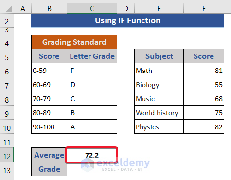
- Then press the Enter key to get the result.
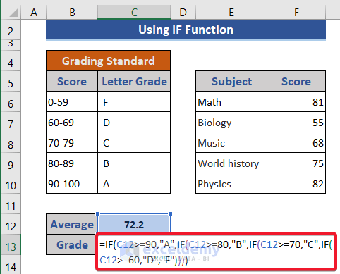
- Now, apply another formula based on the IF function on Cell C13.
=IF(C12>=90,"A",IF(C12>=80,"B",IF(C12>=70,"C",IF(C12>=60,"D","F"))))
- Again, press the Enter button.
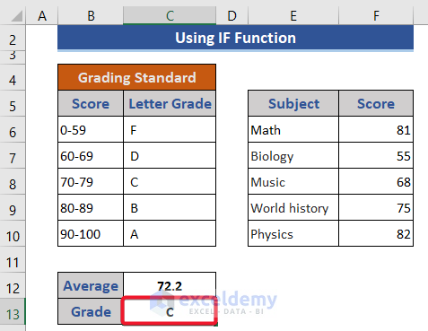
We get the average letter grade easily.
Read More: How to Make Result Sheet in Excel (with Easy Steps)
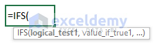
2. Apply IFS Function
We have already found the average score using the AVERAGE function. Now, we will use the Excel IFS function to get the letter grade using the average value.
The IFS function checks whether one or more conditions are met and, returns a value corresponding to the first TRUE condition.
📌 Steps:
- First, directly go to Cell C13 and put the formula based on the IFS function.
=IFS(C12>=90,"A",C12>=80,"B",C12>=70,"C",C12>=60,"D",C12<60,"F")
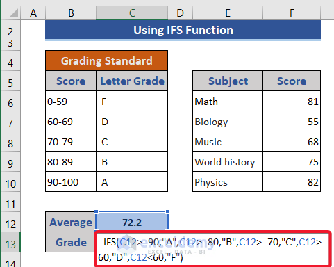
- Press the Enter button to see the result.
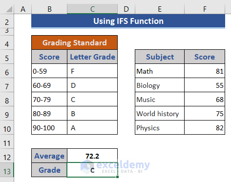
We get the letter grade successfully.
Read More: How to Make a Grade Calculator in Excel (2 Suitable Ways)
Similar Readings
- How to Calculate Final Grade in Excel (with Easy Steps)
- Calculate College GPA in Excel (3 Handy Approaches)
- How to Calculate Subject Wise Pass or Fail with Formula in Excel
- Make Automatic Marksheet in Excel (with Easy Steps)
- How to Calculate Grades with Weighted Percentages in Excel
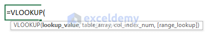
3. Use VLOOKUP Function to Get Average Letter Grades
In this section, we will use the VLOOKUP function using the average value to get the average letter grade.
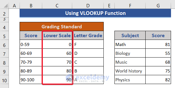
The VLOOKUP function looks for a value in the leftmost column of a table and then returns a value in the same row from a column you specify. By default, the table must be in ascending order.
📌 Steps:
- First, we add a new column in the dataset. This column contains the lower score of each level.
- Now, put the VLOOKUP formula on Cell C13.
=VLOOKUP(C12,$C$6:$D$10,2,TRUE)
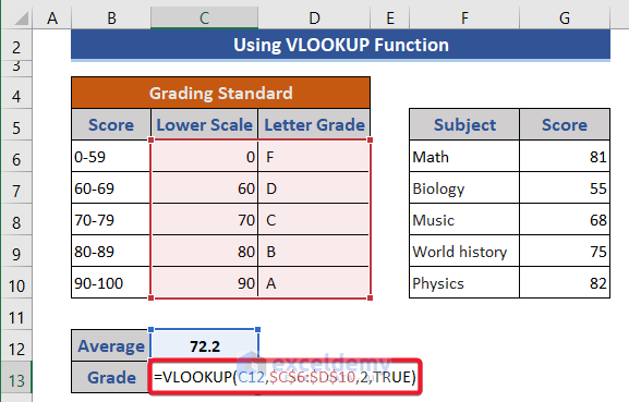
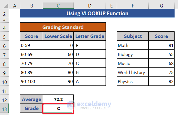
- Then, press the Enter button.
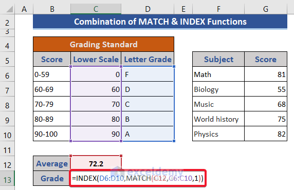
4. Combine MATCH & INDEX Functions
In this section, we will use a combination of the MATCH and INDEX functions. This is a replacement for the VLOOKUP function known widely.
The MATCH function returns the relative position of an item in an array that matches a specified value in a specified order.

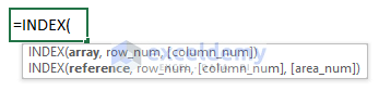
The INDEX function returns a value or reference of the cell at the intersection of the particular row and column, in a given range.
📌 Steps:
- Put the formula based on the combination of the MATCH and INDEX functions on Cell C13.
=INDEX(D6:D10,MATCH(C12,C6:C10,1))
- Finally, press the Enter button to get the result.

Formula Explanation:
- MATCH(C12,C6:C10,1)
This will find a match of C12 in the range C6:C10. If found a value less than C12 in that range then show the row number from the range.
Result: 3
- INDEX(D6:D10,MATCH(C12,C6:C10,1))
This will show the value of the corresponding row from the range D6:D10.
Result: C
Read More: How to Calculate Average Percentage of Marks in Excel (Top 4 Methods)
Conclusion
In this article, we described 4 methods to explain how to get average letter grades in Excel. I hope this will satisfy your needs. Please have a look at our website Exceldemy.com and give your suggestions in the comment box.
Related Articles
- How to Calculate Percentage of Marks in Excel (5 Simple Ways)
- Excel Formula for Pass or Fail with Color (5 Suitable Examples)
- How to Apply Percentage Formula in Excel for Marksheet (7 Applications)
- Calculate Average Percentage Increase for Marks in Excel Formula
- How to Calculate Grade Percentage in Excel (3 Easy Ways)

