8 Steps to Analyse Qualitative Data in Excel
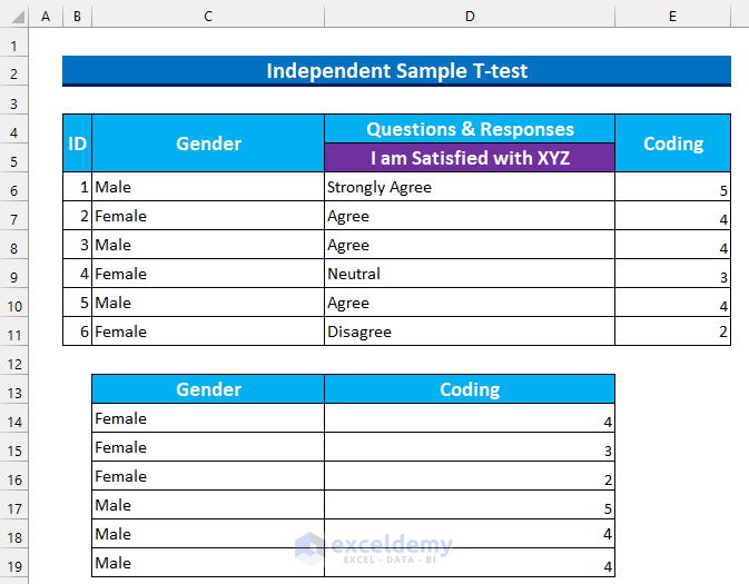
This dataset has 3 columns: “ID”, “Gender”, and “Questions & Responses”.
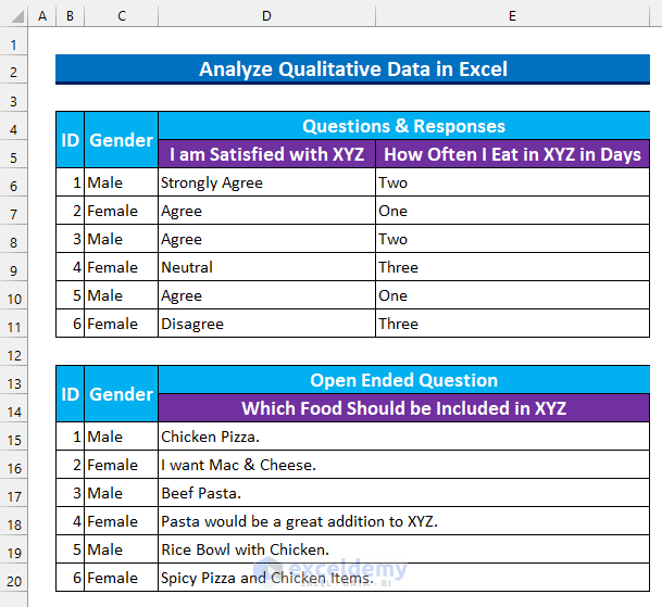
Step 1: Code and Sort Qualitative Data
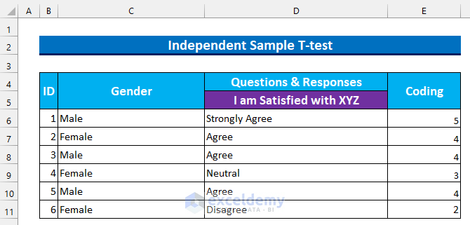
Transform the qualitative data into numerical values using codes. Then, sort the data. Here, the Likert Scale has 5 levels:
- Strongly Agree -> 5.
- Agree -> 4.
- Neutral -> 3.
- Disagree -> 2.
- Strongly Disagree -> 1.
- Input values in the cell range E6:E11.
- Separate the “Gender” and “Coding” columns into different cell ranges.
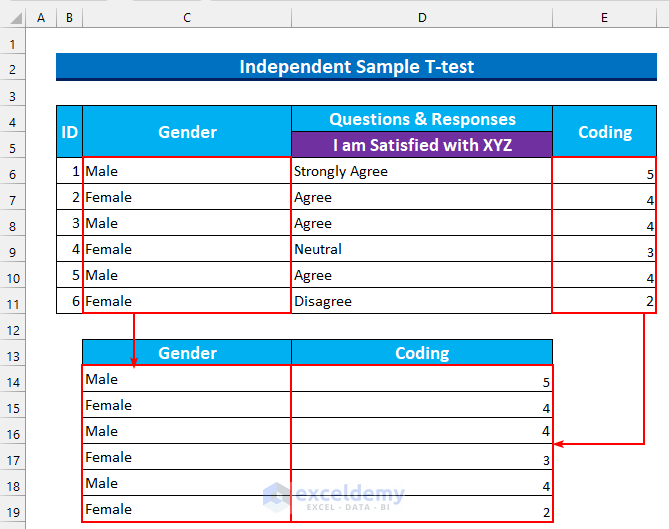
- Select the cell range C14:D19 and right-click to see the Context Menu.
- From Sort >>> select “Sort A to Z”.
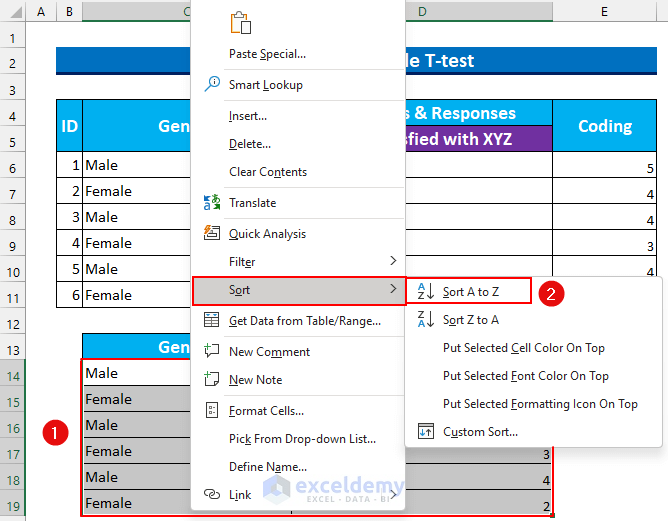
- Values for the same gender will be displayed together.
Read More: How to Analyze Quantitative Data in Excel
Step 2: Enable Analysis Toolpak
- Press ALT, F, then T to open Excel Options.
- From Add-ins >>> select “Go…”.
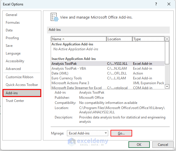
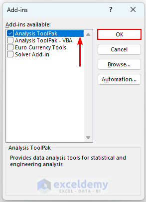
- In the Add-ins dialog box, select “Analysis Toolpak” and click OK.
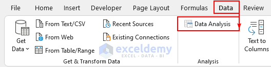
- Data Analysis will be displayed in the Data tab.
Read More: How to Analyse Qualitative Data from a Questionnaire in Excel
Step 3: T-test to Compare Means with Qualitative Data
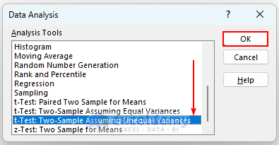
- In Analysis, click “Data Analysis”.
- Select “t-test: Two-Sample Assuming Unequal Variances” and click OK.
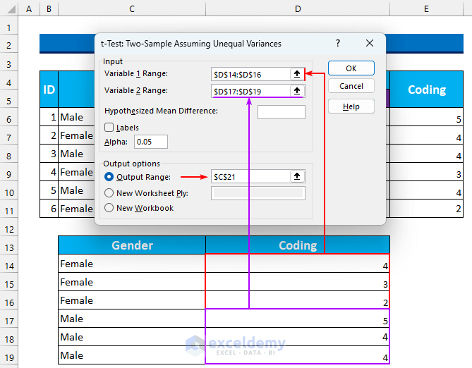
- In the dialog box , select:
- Variable 1 Range – D14:D16.
- Variable 2 Range – D17:D19.
- Select “Output Range” and C21 as the output location.
- Click OK.
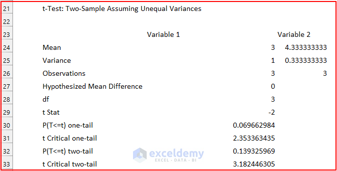
This will be the output.
- The mean is 3 and 4.33. p-value will check wheter this difference is significant. The variances are 1 and 0.33, so the assumption of unequal variances was correct. If this value is almost identical, change it to “t-test: Two-Sample Assuming Equal Variances”.
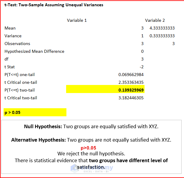
- Focus on the P(T<=t) two-tail value only. It needs to be less than 0.05 to be significant. As it is 0.14 (more than 0.05), reject the null hypothesis.
- The analysis shows that males and females have different levels of satisfaction with cafe XYZ, which is statistically significant.
Step 4: Prepare a Categorical Dataset for a Chi-Square Test
This is the sample dataset.
[/wpsm_box]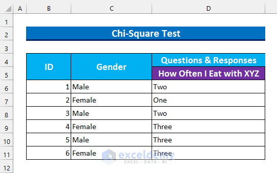
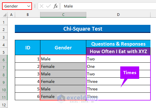
- Name the ranges C6:C11 as “Gender” and D6:D11 as “Times”.
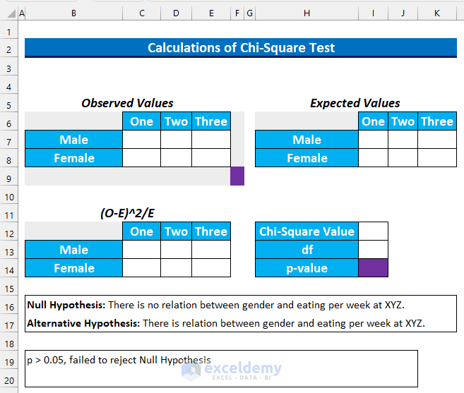
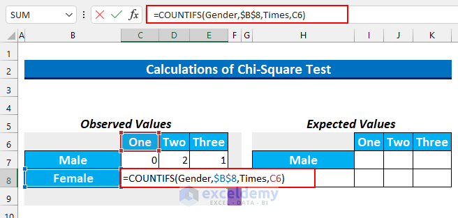
- Create a template to calculate the Chi-Squared value.
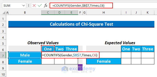
- Select the cell range C7:E7 and enter the following formula.
=COUNTIFS(Gender,$B$7,Times,C6)
This formula finds the number of cells with males and One time eating per week in cafe XYZ.
- Press CTRL+ENTER. This will AutoFill the formula.
- Select the cell range C8:E8 and enter the following formula.
=COUNTIFS(Gender,$B$8,Times,C6)
This formula finds the number of cells containing the females and One time eating per week in cafe XYZ.
- Press CTRL+ENTER.
- Sum the rows and columns.
- Select the cell range C9:E9 and enter this formula.
=SUM(C7:C8)
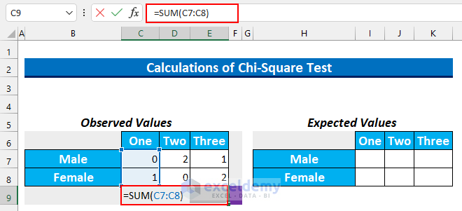
- Press CTRL+ENTER.
- Select the cell range F7:F8 and enter this formula.
=SUM(C7:E7)
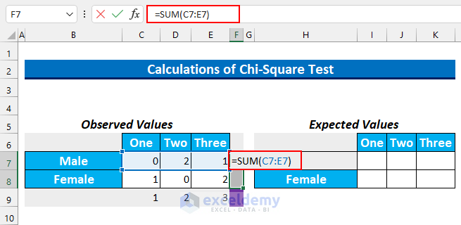
- Press CTRL+ENTER.
- Enter 6 in F9 (the number of respondents).
- To find the expected values, use the formula Row Total * Column Total/Total.
- Select the range I7:K and enter this formula.
=$F$7*C9/$F$9
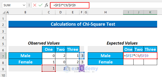
- Press CTRL+ENTER.
- Select the cell range I8:K8 and enter this formula.
=$F$8*C9/$F$9
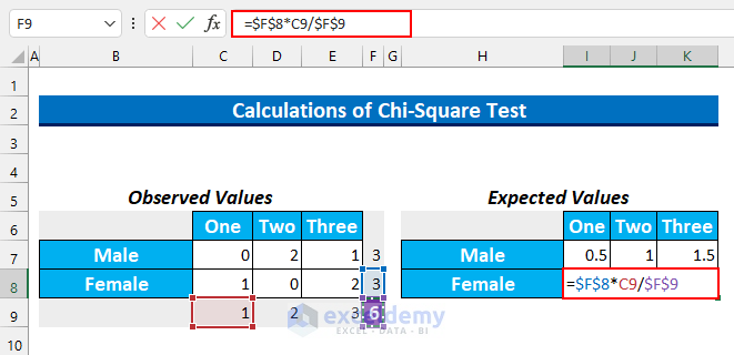
- Press CTRL+ENTER.
- Select the cell range C13:E14 and enter the following formula to find the Chi-Squared value.
=(C7-I7)^2/I7
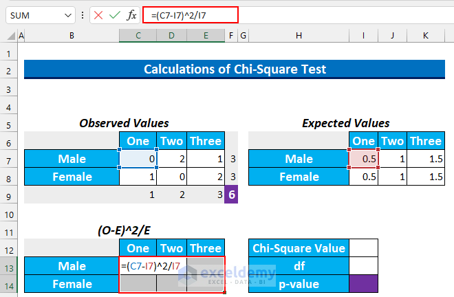
- Press CTRL+ENTER.
- Enter this formula to add these values in I12.
=SUM(C13:E14)
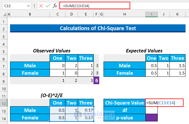
- Press ENTER.
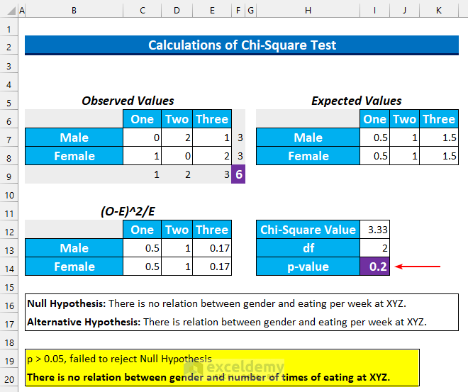
df means degrees of freedom. The formula to find it is (Number of Columns -1) * (Number of Rows-1). There are 2 rows and 3 columns. Therefore, df is (3-1)*(2-1) = 2.
Read More: How to Convert Qualitative Data to Quantitative Data in Excel
Step 5: Analyse Categorical Qualitative Data with a Chi-Square Test in Excel
- Enter this formula in cell I14.
=CHISQ.DIST.RT(I12,I13)
This function returns “the right-tailed probability of the chi-squared distribution”.
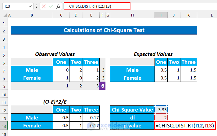
- Press ENTER.
The formula returns 0.2 which is bigger than 0.05. So, the reject the null hypothesis fails: the two categories have no relationship.
Step 6 – Sentiment Analysis for Open-Ended Qualitative Data
Two columns were added to the dataset: “Topic1” and “Topic2”.
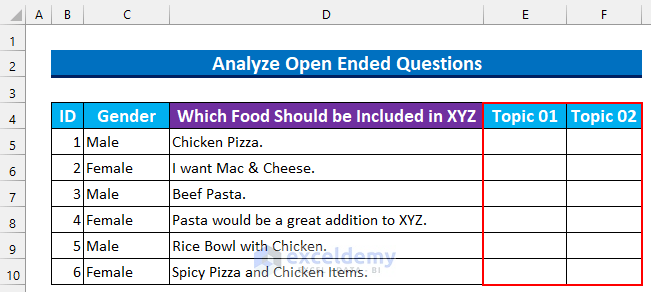
- You should read the responses and link them to food topics. For example, “Chicken Pizza” has 2 topics: “Chicken” and “Pizza”.
- Each topic is then added to a new table.
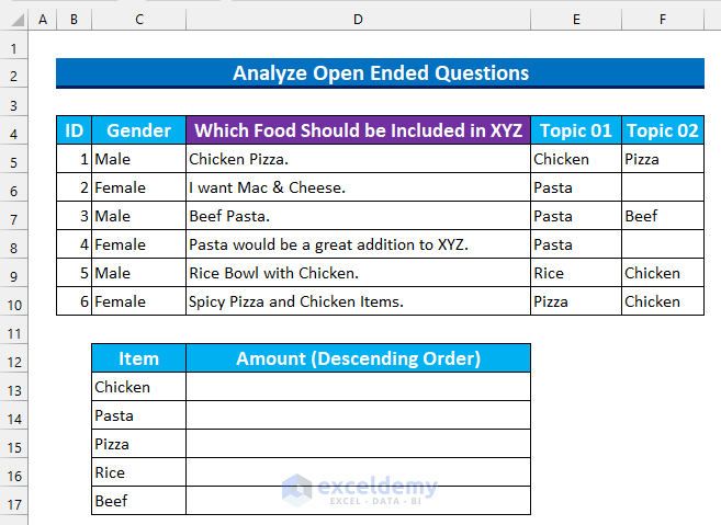
Step 7 – Use the COUNTIF Function to Analyse Open-Ended Qualitative Data
- Select the cell range D13:D17 and enter the following formula.
=COUNTIF($E$5:$F$10,C13)
This formula counts the number of values in the range F5:F10 that match the value in C13.
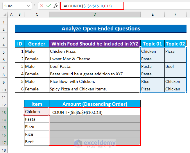
- Press CTRL+ENTER to AutoFill the formula.
- Insert a Chart to see the frequency distribution.
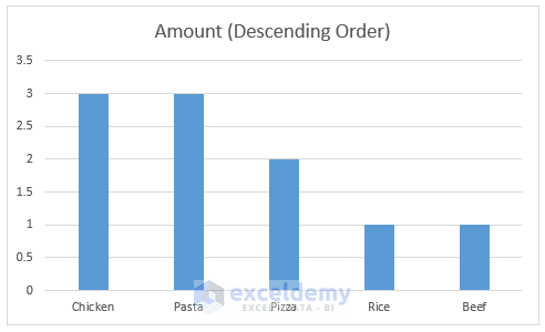
Step 8 – Using a Clustered Column Chart to Visualize Open-Ended Qualitative Data
- Select the cell range C12:D17.
- From the Insert tab, select Recommended Charts.
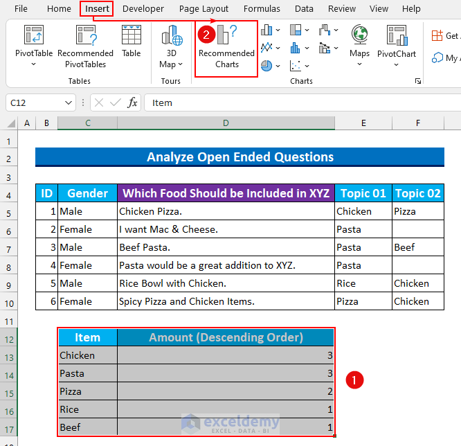
- In the Insert Chart dialog box, select Clustered Column (it may be selected by default).
- Click OK.

The top 3 food items in XYZ cafe are Chicken, Pasta, and Pizza.
Read More: How to Analyze Raw Data in Excel
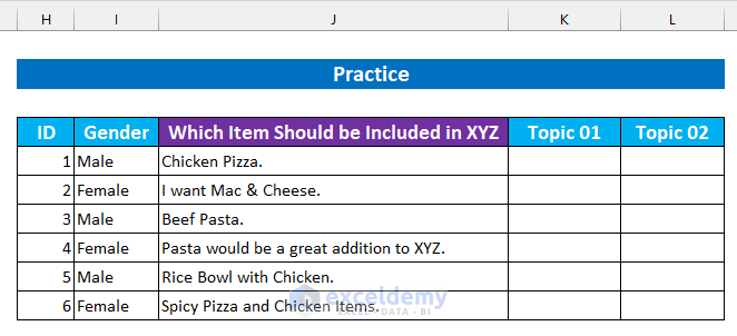
Practice Section
Practise with the following dataset.
Related Articles
- How to Analyze Large Data Sets in Excel
- How to Analyze Text Data in Excel
- How to Analyze Time Series Data in Excel
- How to Analyze Sales Data in Excel
- How to Analyze Likert Scale Data in Excel
- How to Analyze qPCR Data in Excel
- How to Analyze Time-Scaled Data in Excel
<< Go Back to Data Analysis with Excel | Learn Excel
Get FREE Advanced Excel Exercises with Solutions!
