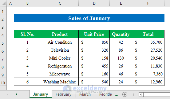
In the sample dataset you have the sales of January, February, and March in different sheets. This sheet contains the Sales of January.
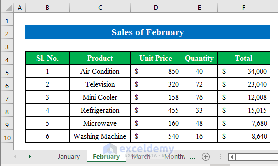
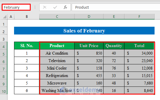
- These are the Sales of February.
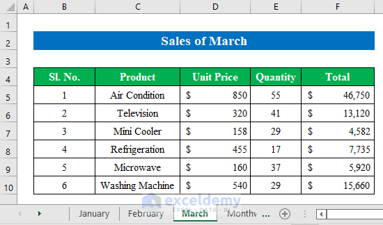
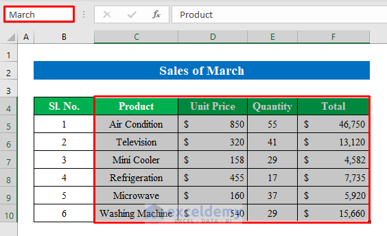
- These are the Sales of March.
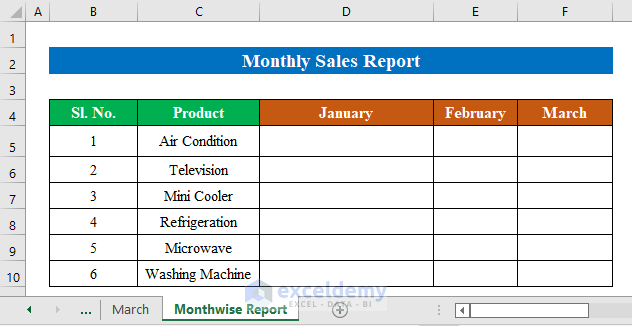
- Open a new worksheet to calculate the monthly sales report for each item.
Step 1 – Define the Range for Each Month
- Select cells (C4:F10).
- Enter “January” in the name box.
- Press Enter to continue.

- Open another sheet and select the data range. Here, (C4:F10).
- Enter “February” in the name box.
- Press Enter.
- Open a new sheet “March” and follow the previous steps.
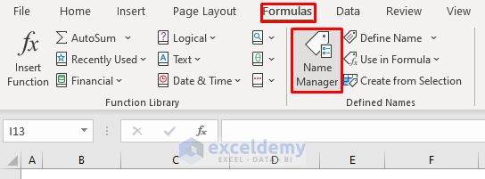
- Go to “Formulas” and click “Name Manager”.
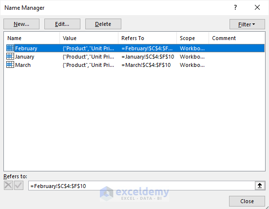
- In the “Name Manager” window, edit the range or the names.
Read More: How to Make Monthly Report in Excel
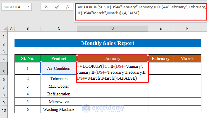
Step 2 – Applying a Formula to Make a Monthly Sales Report
- Select a cell. Here, (D5).
- Enter the formula:
=VLOOKUP($C5,IF(D$4="January",January,IF(D$4="February",February,IF(D$4="March",March))),4,FALSE)Where,
- The VLOOKUP function looks for information in a data range or string.
- The IF function returns one value if true and another value if false within a given condition. In the Table Array (D$4=”January” – if it’s true it will collect data from “Sales of January”. If false then it will go to “February” or “March”.
- Col_index_num is 4, and shows the total sale of each item.
- To return an exact match for your lookup value, select FALSE.
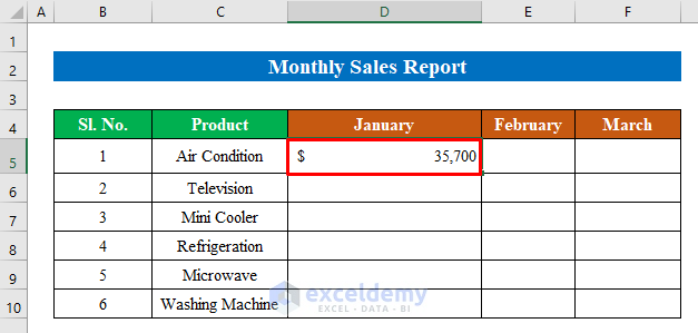
- Press Enter to see the output.
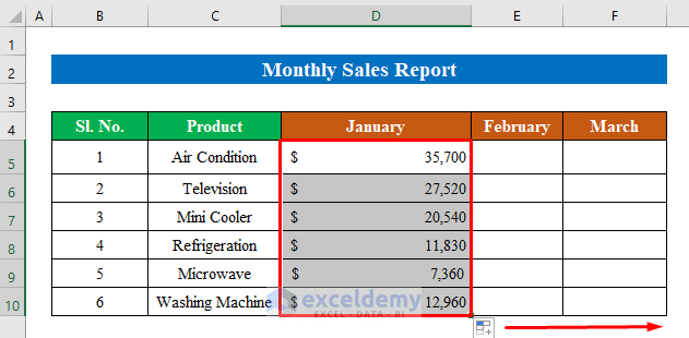
- Drag down the “fill handle” to see the result for all items in the column.
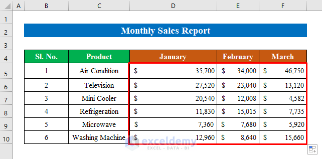
- Drag it to the right to see the result for February and March.
- This is the monthly sales report.
Read More: Create a Report That Displays Quarterly Sales in Excel
Download Practice Workbook
Download this practice workbook to exercise.
- How to Prepare MIS Report in Excel
- How to Make MIS Report in Excel for Accounts
- How to Make Daily Sales Report in Excel
- How to Make MIS Report in Excel for Sales
- Create a Report that Displays the Quarterly Sales by Territory
- How to Make Sales Report in Excel
<< Go Back to Report in Excel | Learn Excel
Get FREE Advanced Excel Exercises with Solutions!

HELLO, HOW TO SOLVE THESE PROBLEMS IN EXCEL?
1.Five girls are in bakery business, and they want to check how they have done sales in every month.
2.They have different products like Cake, Pies, Sandwich, Bread, Burger, and Donuts.
3.Please create pie chart to understand which product is sold high and low by all the ladies
4.If the sales of cakes are more than 100, that lady is announcing 10% discount for the next month
5.Ladies with only 5 letters in their name are allowed to use data validation for their cake products
Dear FODAY,
Thank you for your response. As per your query-
1. You can create a Pie Chart to visualize the sales from the “Insert” option.
Imagine a dataset with multiple Bakery Products and their Total Sales. Now we will create a pie chart using the information from the dataset.
First, select the products and total sales column and then press “Recommended Chart” from the “Insert” option.
Second, from the new dialog box choose “Pie Chart” and press OK to continue.
Finally, within a moment your final pie chart will be in your hands showing sales of multiple products.
2. As per your second query-
We will use the IF function to calculate the “10%” discount price if the sales of cake is more than 100.
To do that choose a cell (G5) and write the following formula down-
=IF(E5>100,(D5-(D5*0.1)),D5)Hence, hit Enter and the final output will be in your hands.
3. Now coming to the last query you wanted to use the data validation for ladies with only 5 letters in their name. Well, below I have shared the simplest solution.
Suppose we have a dataset with some Lady Names. Now we will use data validation for the name list.
First, selecting the names from the list click the “Data Validation” option from the “Data” feature.
Second, click “Settings” and choose criterias according to the screenshot and press OK to continue.
Finally, we have applied data validation over the name list. To check try editing any names not fulfilling the condition and you will get a notification about “This Value doesn’t match the data validation restrictions defined for this cell.”