Method 1 – Utilizing a PivotTable to Make a MIS Sales Report
Steps:
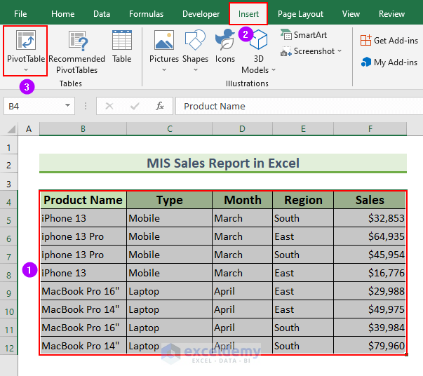
- Select the cell range B4:F12.
- From the Insert tab, select PivotTable.
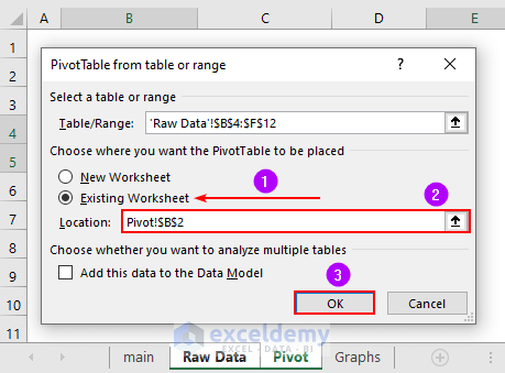
A dialog box will appear.
- Select Existing Worksheet and cell B2 in the “Pivot” Sheet as the output location.
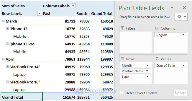
We’ll see the PivotTable Fields dialog box.
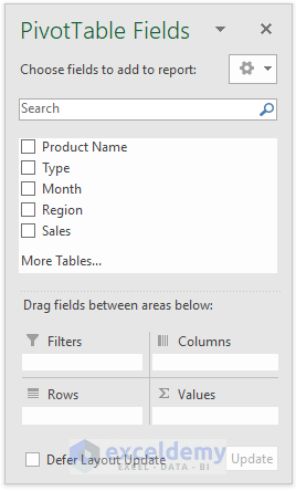
- Select all the Fields. This will put everything except the Sales fields into Rows.
- Drag the “Region” field to Columns.
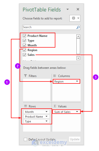
You should get an output similar to this.
Method 2 – Inserting Charts in Excel
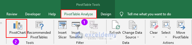
- Select anywhere on the PivotTable output data.
- From PivotTable Analyze, select PivotChart.
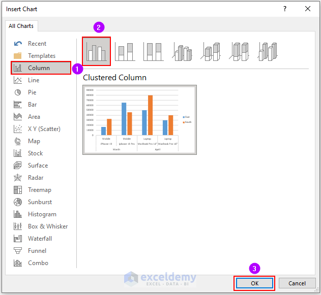
The insert Chart dialog box will appear.
- From Column, select Clustered Column.
- Press OK.
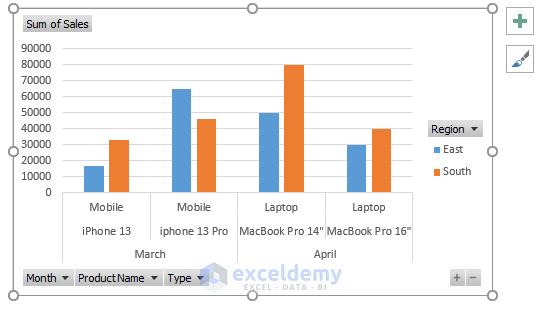
You’ll see a column Chart on the Sheet.
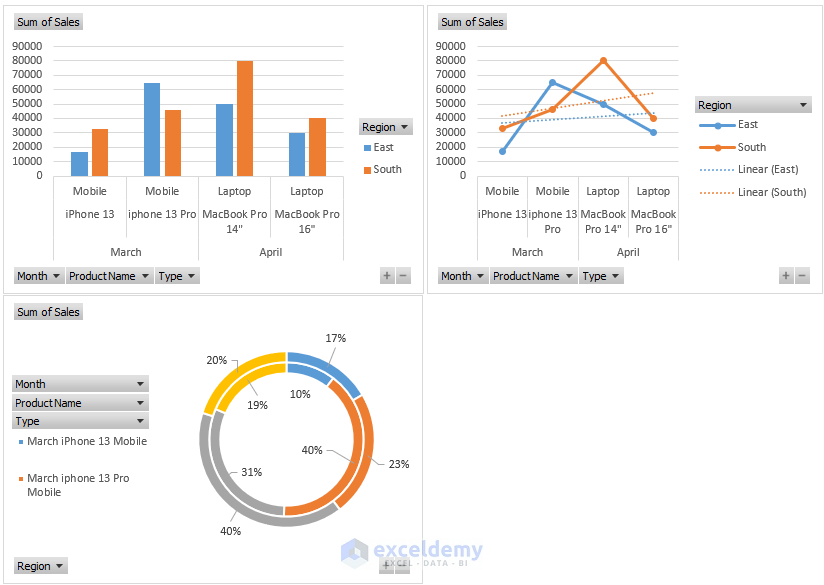
Graph Breakdown
- The iPhone 13 is more profitable in the South region.
- The demand is higher for iPhone 13 Pro in the East region.
- For laptops, both models of MacBook are more prevalent in the South region.
- The company should increase the inventory of iPhone 13 for South, iPhone 13 pro for East, and Laptops for the South region.
Add a Pie Chart.
- From the PivotTable Analyze, select PivotChart.
- From Pie, select Doughnut and press OK.
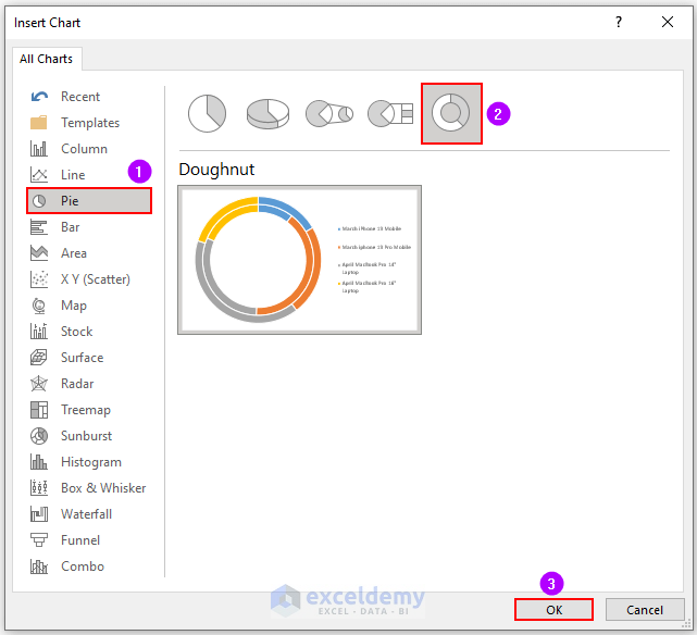
A Doughnut type Pie Chart will be shown.
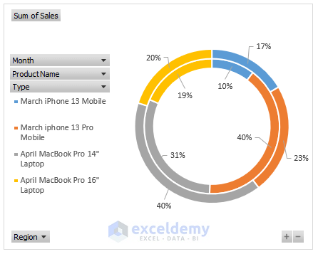
Graph Breakdown
- The outer ring is for the South region.
- Consider the Product Types, then Laptop accounts for 60% and 50% of Total Sales for the South and East region respectively.
- The higher model of the MacBook is twice as popular as the Base model in the South Region.
- In the East region, iPhone 13 Pro is 4 times as popular as the iPhone 13.
Add Line Chart.
- From PivotTable Analyze, select PivotChart.
- From Line, select “Line with Markers” and press OK.
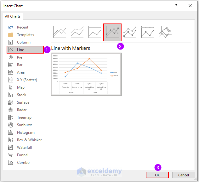
- A “Line Graph” will appear.
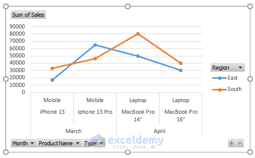
Graph Breakdown
- For Mobiles, the higher model has generated more sales. However, this is not true for Laptops.
- The East region accumulated more sales with Mobile phones.
- The South region gained more revenue for the base Laptop model.
- The company may drop the MacBook Pro 16” model from its product portfolio.
Method 3 – Moving Charts to Another Sheet
- Select any of the three charts.
- From PivotChart Analyze, select Move Chart.
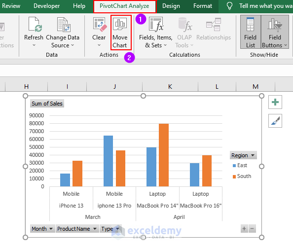
The Move Chart dialog box will appear.
- From Object in, select Graphs.
- Press OK.
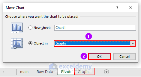
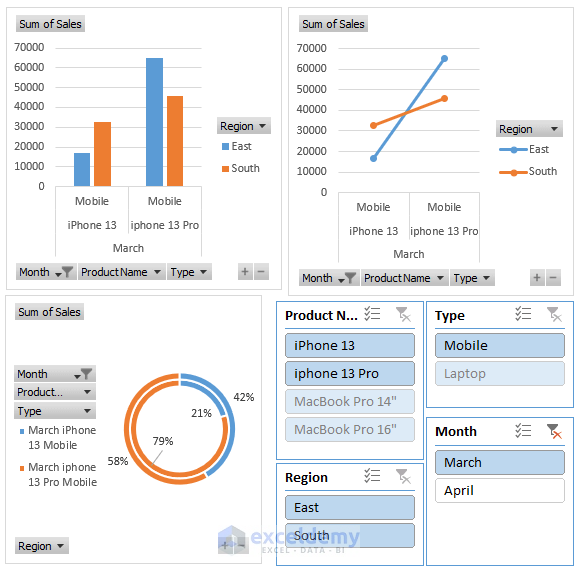
Move all the Charts to the new Sheet.
Laying Slicers in Excel to Make MIS Sales Report
Add Slicers. This will allow us to apply Filters to our Charts.
- Select any of the Graphs.
- From the PivotChart Analyze tab, select “Insert Slicer”.
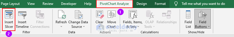
A dialog box will appear.
- Select the first 4 fields and click OK.
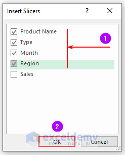
The Slicers will look like this.
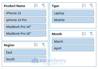
Click on any of the fields to change our datasets.
- Select “March” under the Month Slicer.
This will show only the values from the month of March.
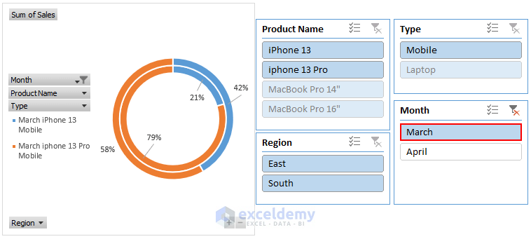
Our Slicer will modify all the existing Charts. We’ve created an MIS sales report in Excel.
Download the Practice Workbook
Related Articles
- How to Prepare MIS Report in Excel
- How to Make MIS Report in Excel for Accounts
- Create a Report that Displays the Quarterly Sales by Territory
- How to Make Daily Sales Report in Excel
- Create a Report That Displays Quarterly Sales in Excel
<< Go Back to Report in Excel | Learn Excel
Get FREE Advanced Excel Exercises with Solutions!
