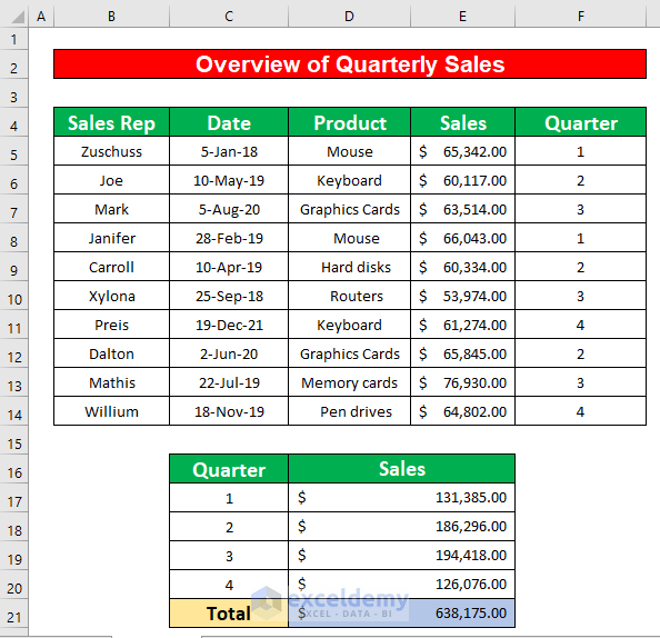
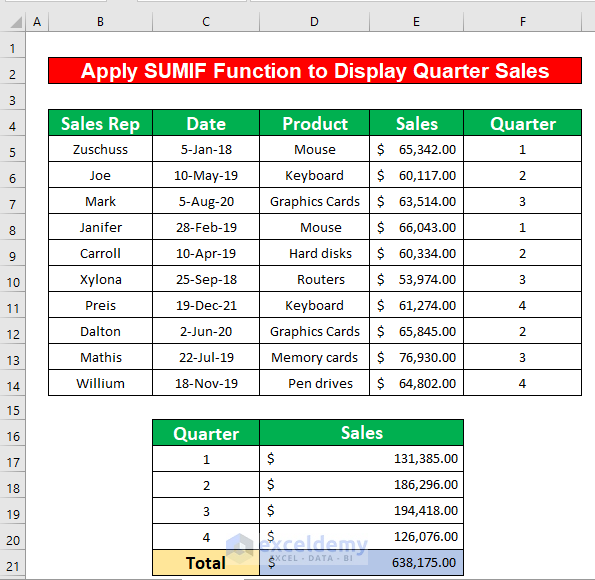
We have a worksheet that contains information on sales representatives, products, selling dates, and sales. Here’s the overview of the sheet we’ll make with the information.
Step 1 – Combine CHOOSE and MONTH Functions to Determine Quarterly Sales
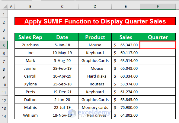
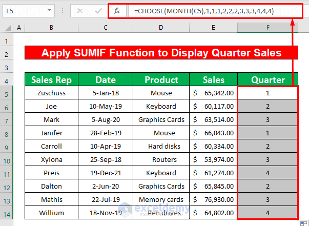
- Select cell F5.
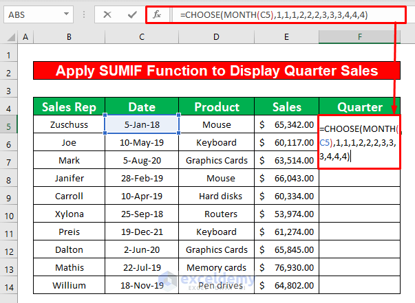
- Insert the following formula:
=CHOOSE(MONTH(C5),1,1,1,2,2,2,3,3,3,4,4,4)Formula Breakdown:
- C5 is the serial_num of the MONTH function.
- MONTH(C5) is the index_num of the CHOOSE function, and 1,1,1,2,2,2,3,3,3,4,4,4 is the value of month number.
- Press Enter.
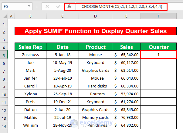
- AutoFill the formula to the rest of the cells in column F.
Read More: How to Make Daily Sales Report in Excel
Step 2 – Apply the SUMIF Function to Get Total Quarterly Sales
- Select the cell D17 and apply the following function in that cell.
=SUMIF(F5:F14,C17,E5:E14)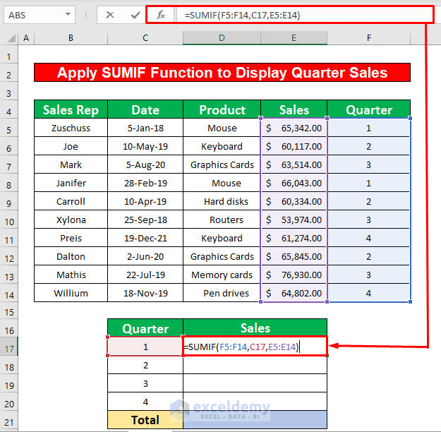
- Press Enter.
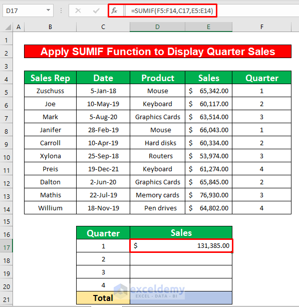
- AutoFill the function to the rest of the cells in column D.
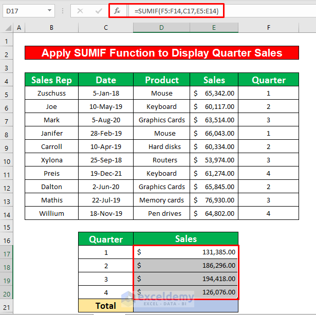
- Sum up the sales from the different quarters in cell D21.
Step 3 – Create a Pie Chart to Display a Quarterly Sales Report in Excel
- Select the data range. We will select cells D17 to D20 for the convenience of our work.
- From the Insert tab, go to Chart and select Insert Pie.
- Select 2-D Pie.
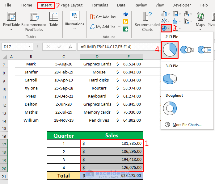
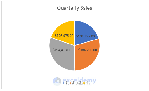
- You will get a 2-D Pie chart.
Read More: How to Make Sales Report in Excel
Download the Practice Workbook
Related Articles
- How to Prepare MIS Report in Excel
- How to Make MIS Report in Excel for Accounts
- How to Make MIS Report in Excel for Sales
- Create a Report that Displays the Quarterly Sales by Territory
- How to Make Monthly Sales Report in Excel
<< Go Back to Report in Excel | Learn Excel
Get FREE Advanced Excel Exercises with Solutions!
