How to Make a Monthly Expense Report in Excel (With Quick Steps)

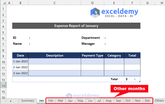
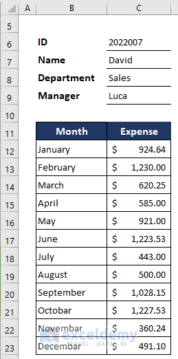
Step 1: Design a Preliminary Summary Layout

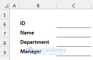
• In the range of cells B6:B9, enter the following entities, as shown in the image.
• Format the range of cells C6:C9 according to your desire to input the employee’s data.

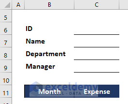
• Name cells B11 and C11 as Month and Expense.

• Enter all the months in the range of cells B12:B23.

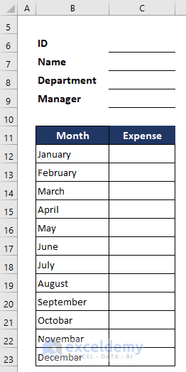
• Our preliminary summary layout is ready.

Step 2: Create a Monthly Expense Report for All Months

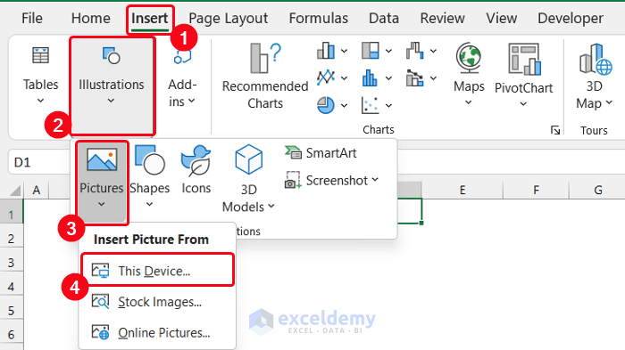
• Select cell D1 to insert your company logo.
• In the Insert tab, click the drop-down arrow of Illustrations > Pictures.
• Select the This Device option.

• The Insert Picture dialog box will appear. Choose your organization’s logo. We are inserting our webpage logo for your convenience.
• Click the Insert button.

• The logo will be inserted and placed the logo at your desired location.

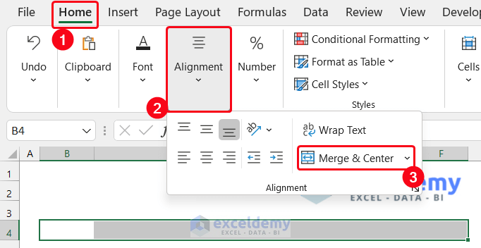
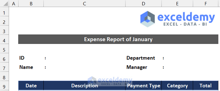
• Select the range of cells B4:F4.
• Select the Merge & Center option from the Alignment group in the Home tab.

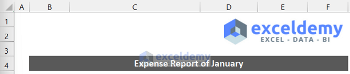
• In the merged cell, set a suitable title for the sheet. We denote the sheet as the January Expense Report.

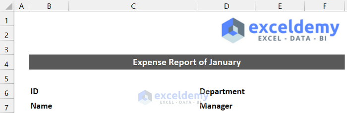
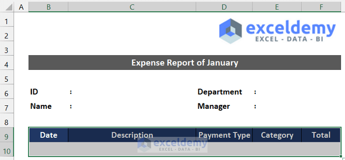
• In the range of cells B6:B7 and D6:D7, enter the following entities.

• Select cell C6 and enter the following formula to extract the employee’s ID from the Summary:

• Press Enter.

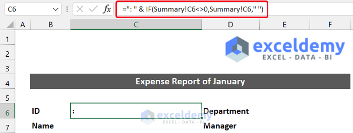
• Here, we have used the IF function to get a good cell formatting.
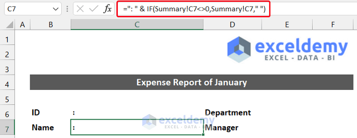
• In cell C7, enter the following formula to get the name of that employee:

• Press Enter.

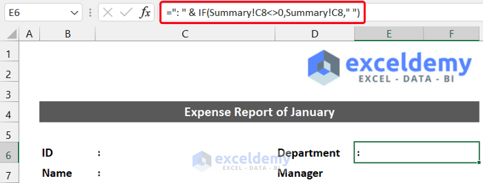
• In cell E6, enter the formula to get the value for the department name:

• Press Enter.

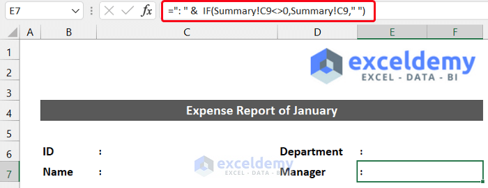
• In cell E7, enter the following formula to get the manager’s name:

• Then, press Enter.

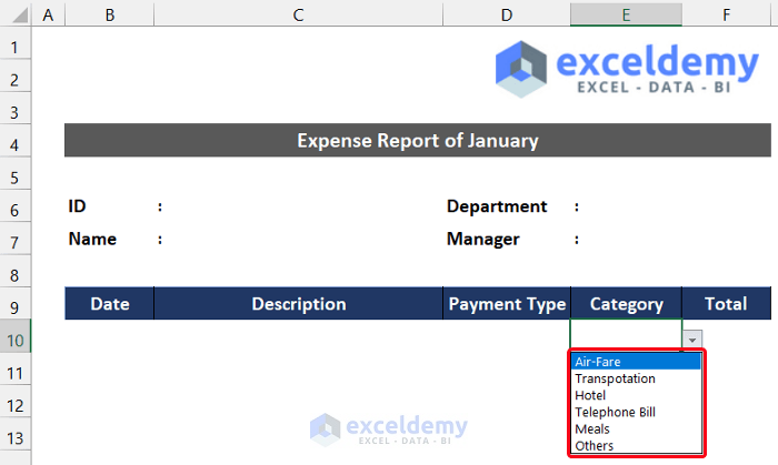
• For the monthly expense table, enter the following titles in the range of cells B9:F9, as shown in the image.

• Use the data validation feature to ensure the proper data is input in columns Payment Type and Category.
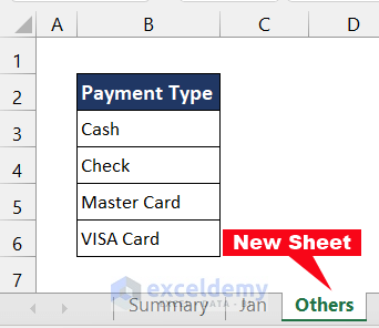
• Create a separate sheet and rename it as Others.
• In the range of cells B3:B6, enter the four types of payment systems.

• Select cell D10, and in the Data tab, select the drop-down arrow of Data Validation > Data validation from the Data Tools group.

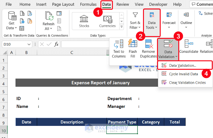
• A small dialog box called Data Validation will appear.
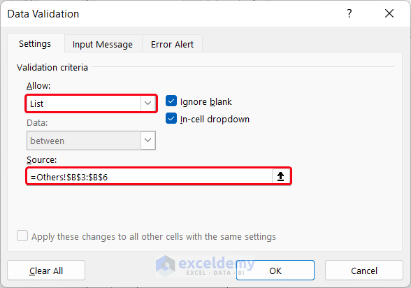
• Set the Allow option as List, and in the Source option, select the range of cells Others!$B$3:$B$6.
• Click OK.

• In cell E10, create the same data validation drop-down for the categories shown in the Others sheet in the range of B9:B14.

• Convert the dataset into a table. It will help you copy the data validation drop-down arrow in every new row of this table.
• Select the range of cells B9:F10 and press ‘Ctrl+T’ to convert the dataset into a table.

• The Create Table dialog box will appear.
• Check the My table has headers option and click OK.

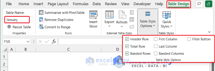
• In the Table Design tab, set the table name as January from the Properties group.
• Modify the Table Style Options according to your desire. We checked the following items for our table.

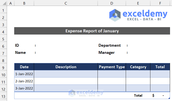
Our monthly expense data table for January is ready to use.

• Follow the procedure to create the monthly expense sheet for the rest of the month.

Step 3: Verify the Summary Report with Data

• Input the following data according to your institution profile in the range of cells C6:C9.

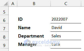
• You will see the IF function, which will show these data in our monthly expense sheet.
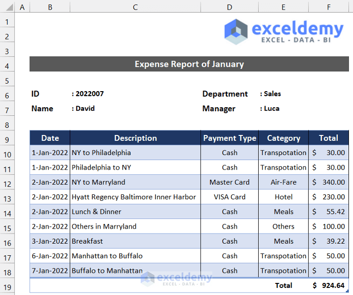
• Input some sample data into the January table, as shown in the image below.

• In the Summary sheet, select cell C12 and enter the following formula into the cell:

• Press Enter.

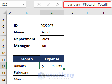
• Enter is a similar formula to extract each month’s total expense in the range of cells C13:C23.

• Our summary report is completed.

Step 4: Generate a Dynamic Monthly Expense Report

• In the Summary sheet, select the range of cells B12:C23.
• In the Insert tab, select the drop-down arrow of the Insert Pie or Doughnut Chart option and select the 3-D Pie option.

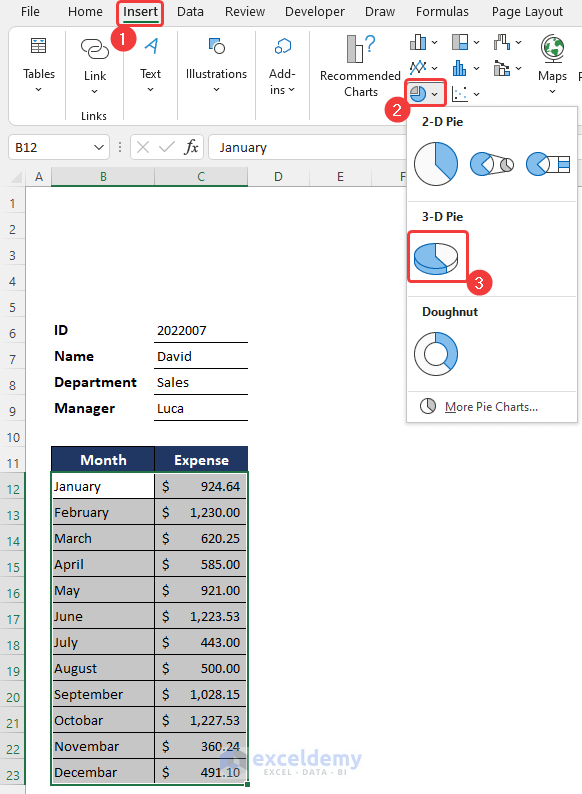
• The chart will appear.
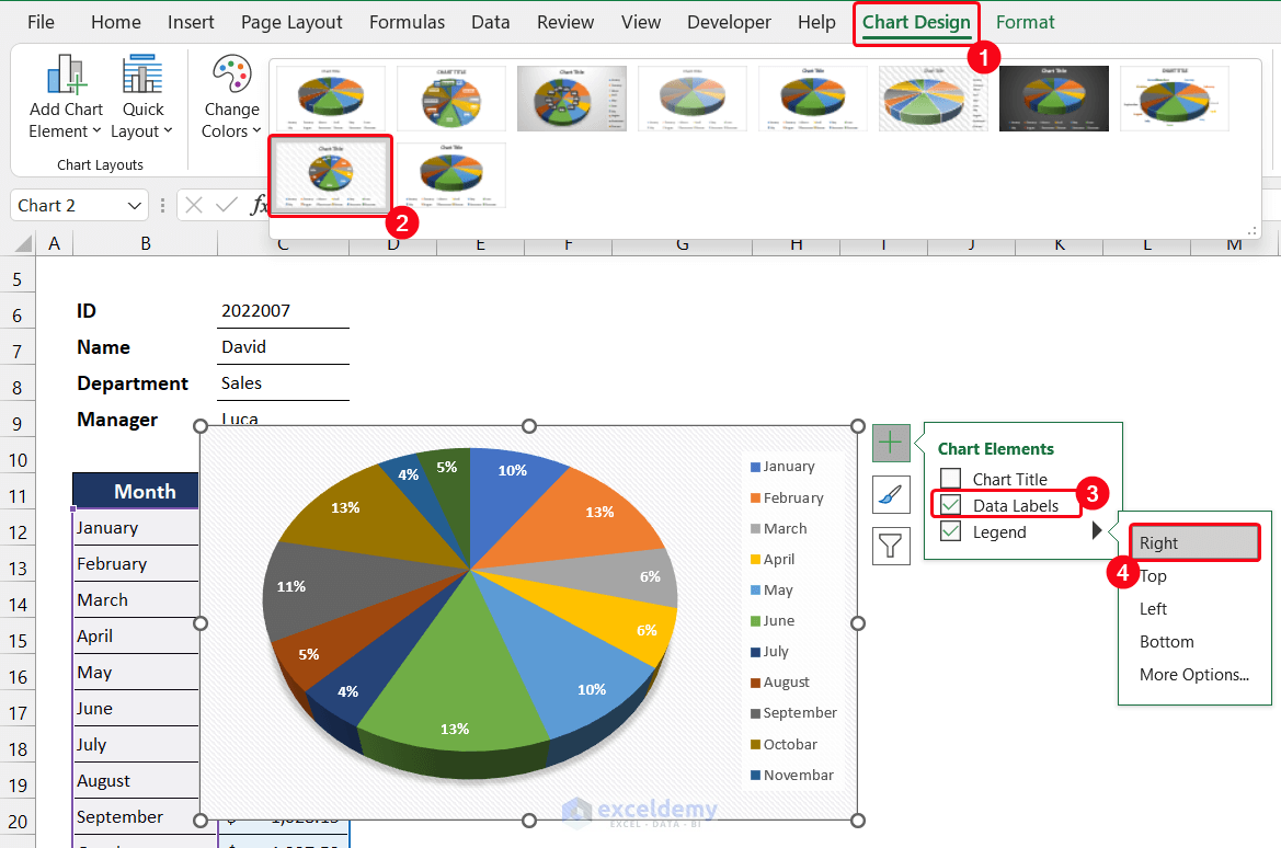
• You can modify the chart style from the Chart Design and Format tabs. We chose Style 9 from the Chart Styles group for our pie chart.
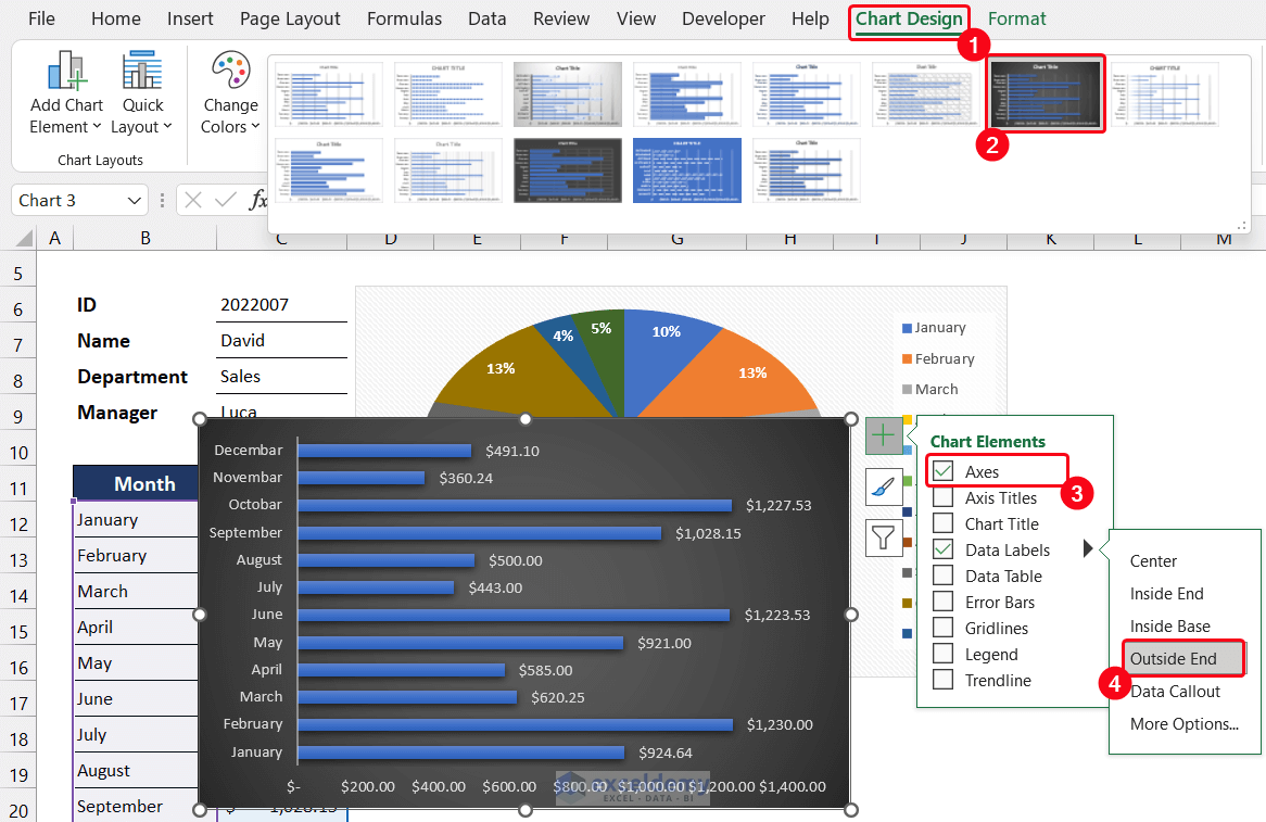
• Click on the Chart Elements icon and check the Data Labels.
• Place the Legends on the right side.

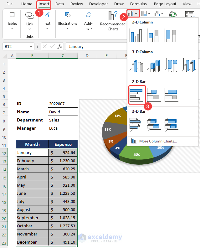
• Select the range of cells B12:C23.
• To insert the Bar chart, follow the same process, and in the drop-down arrow of Columns or Bar Chart, select the Clustered Bar option from the 2-D Bar section.

• You can modify the number of elements and the chart style according to your preference. We chose Style 7 and this chart’s Axes and Data Labels elements.
• To show the Data Labels, choose the Outside End option.

• Place both charts in a suitable position on the summary sheet.
• Select the range of cells B4:J4, and in the Home tab, click on the Merge & Center option from the Alignment group.

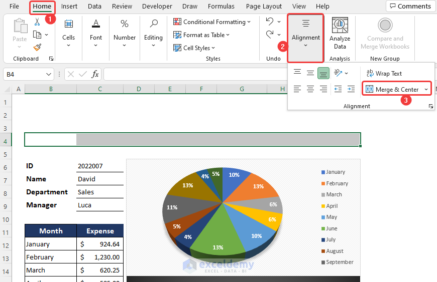
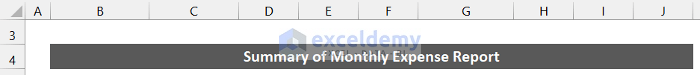
• Enter a suitable title into the merged cell according to your desire. We wrote down the Summary of Monthly Expense Report as the title for our sheet.

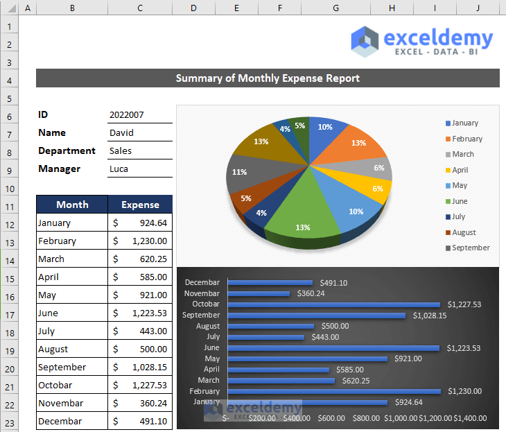
• Follow the same process as step 2 to insert your organization’s logo in cell G1.
• Our monthly expense report is completed and ready to use.

Download the Practice Workbook

Download this free workbook to practice.

Related Articles

• How to Create an Expense Report in Excel
• How to Make Production Report in Excel
• How to Make Daily Production Report in Excel
• How to Create an Income and Expense Report in Excel
• How to Make Daily Activity Report in Excel
• How to Make Monthly Report in Excel

<< Go Back to Report in Excel | Learn Excel