In this article we will demonstrate step-by-step procedures to create a daily, weekly and monthly income and expense report in Excel.
Watch Video – Create an Income and Expense Report in Excel
Example 1 – Daily Income and Expense Report
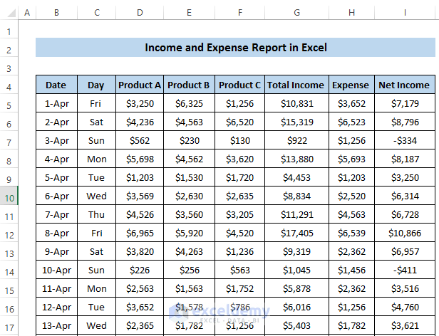
Step 1 – Import Dataset
To start with, we need to import or create a dataset from which to create the report. For this example, we’ll use the dataset below that contains an income and expense report of a company selling 3 products. The sum of the Income from these products minus the daily Expenses give a Net Income for each day.
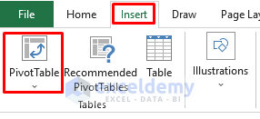
Step 2 – Create Pivot Table
Now we’ll use this dataset to create a Pivot Table.
- Select your whole dataset by clicking on any cell in it and pressing Ctrl+A.
- Go to the Insert tab on the ribbon.
- Select PivotTable.
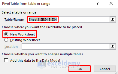
The PivotTable from table or range dialog box will pop up.
- As the entire dataset was pre-selected, it should already be filled in the Table/Range option.
- Choose New Worksheet to place the PivotTable in a new worksheet.
- Click on OK.
- Go to the worksheet where your PivotTable is located.
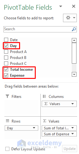
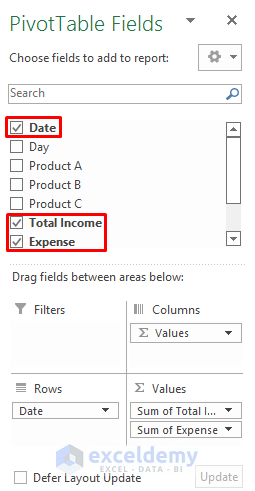
On the right is a PivotTable Fields section.
- Select Day, Total Income, and Expense.
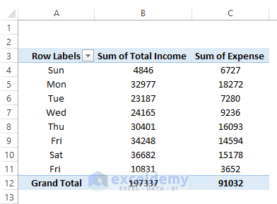
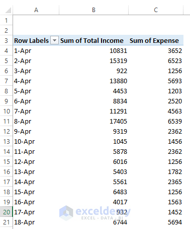
PivotTable will generate the following table with the selected column headers.
Step 3 – Insert Daily Income and Expense Report Chart
For better visualization, we’ll now plot this data into a chart.
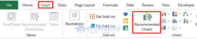
- Select any cell in the Pivot Table.
- Go to the Insert tab on the ribbon.
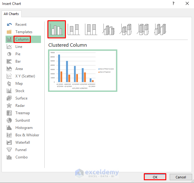
- From the Chart group, select Recommended Charts.
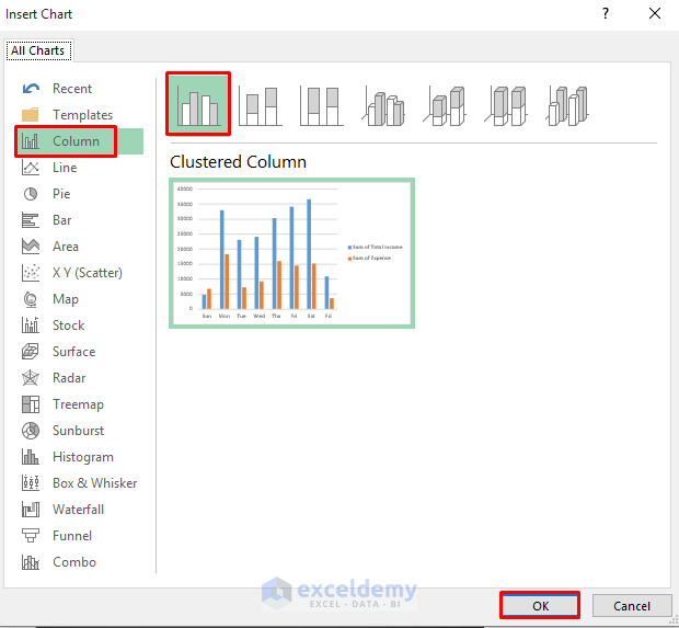
The Insert Chart dialog box will appear.
- Select the Column chart from the All Chart section.
- Select a column chart, for example the first one.
- Click on OK.
Our chart is created.
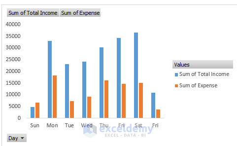
- Modify the chart by using the Brush and Plus sign.
- The Brush sign can change the chart style.
- The Plus sign can change the chart elements.

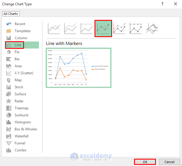
Suppose instead of a column chart we want to use a line chart.
- Select any cell in the Pivot Table.
- From the Chart group, select Recommended Charts.
The Insert Chart dialog box will appear.
- Select the Line chart from the All Chart section.
- Select a chart, for example the fourth Line chart.
- Click on OK.
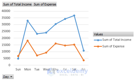
We have our desired line chart.
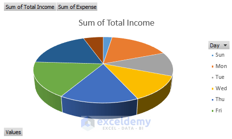
To create a pie chart is more or less the same process:
- Go to the Insert tab on the ribbon.
- From the Charts group, select Recommended Charts.
The Insert Chart dialog box will appear.
- Select the Pie chart from the All Charts section.
- Select a chart, for example the second Pie chart.
- Click on OK.
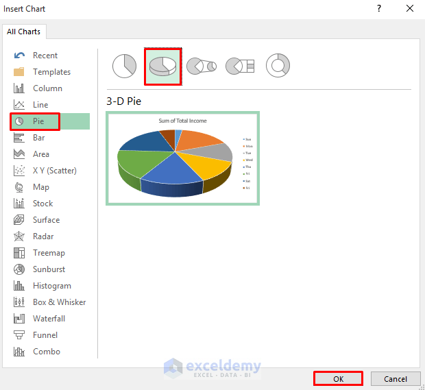
We have our desired Pie chart.
Finally, we’ll create a Combo chart.
- Go to the Recommended Charts option like for the previous charts.
The Insert Chart dialog box will appear.
- Select the Combo chart from the All Charts section.
- Select a chart, for example the fourth Combo chart.
- Click on OK.
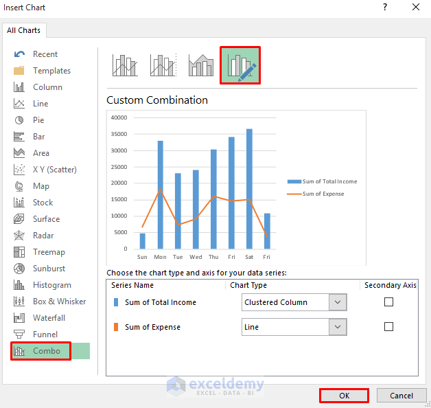
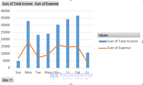
This will create a Combo chart like the following:
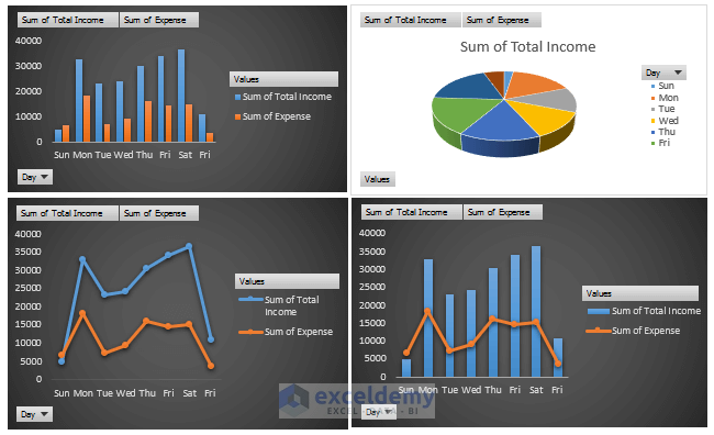
Step 4 – Create Final Daily Income and Expense Report
When you’re done plotting daily income and expenses in different chart types, copy them and paste them into a new worksheet, presented in the following way:
Read More: How to Make Daily Sales Report in Excel
Example 2 – Weekly Income and Expense Report in Excel
Now we’ll create a weekly income and expense report.
Step 1 – Import Dataset
As before, we need to import a dataset from which to create the report. We’ll use the same dataset as above to illustrate this example too.
Step 2 – Create Pivot Table
Now we create a Pivot Table from the dataset,
- Select the whole dataset by selecting any cell in it and then pressing Ctrl+A.
- Go to the Insert tab in the ribbon.
- Select PivotTable.
The PivotTable from table or range dialog box will pop up.
- The Table/Range option should be pre-filled with the selected range of cells.
- Choose New Worksheet to place the PivotTable in a new worksheet.
- Click on OK.
- Go to the worksheet where the PivotTable is located.
On the right is the PivotTable Fields section.
- Select Date, Total Income, and Expense.
The PivotTable will provide the following table with the selected column headers.
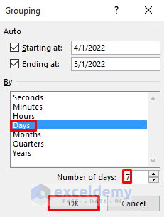
- Right-click on any cell in the “day” column.
- From the context menu, select Group.

A Grouping box will appear.
- Select Days as the By option.
- Set the Number of days to 7.
- Click on OK.
Step 3 – Insert Weekly Income and Expense Report Chart
Now we’ll generate and insert the charts.
- Select any cell in the Pivot Table.
- Go to the Insert tab on the ribbon.
- From the Chart group, select Recommended Charts.
The Insert Chart dialog box will appear.
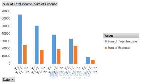
- Select the Column chart from the All Chart section.
- Select a chart, for example the first Column chart.
- Click on OK.
Our desired chart is inserted.
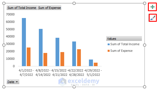
- Modify the column chart by using the Brush and Plus sign.
- The Brush sign can change the chart style.
- The Plus sign can change the chart elements.
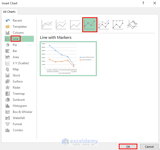
Next, we’ll generate a Line chart.
- Select any cell in the Pivot Table.
- From the Charts group, select Recommended Charts.
The Insert Chart dialog box will appear.
- Select the Line chart from the All Charts section.
- Select a chart, for example the fourth Line chart.
- Click on OK.
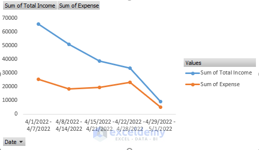
Our desired line chart is inserted.
Now, a Pie chart:
- Go to the Insert tab on the ribbon.
- From the Charts group, select Recommended Charts.
The Insert Chart dialog box will appear.
- Select the Pie chart from the All Charts section.
- Select a chart, for example the second Pie chart.
- Click on OK.
There we have our desired Pie chart.
Finally, let’s create a Bar chart.
- Go to the Recommended Charts option like for the previous charts.
The Insert Chart dialog box will appear.
- Select the Bar chart from the All Charts section.
- Select a char, for example the first Bar chart.
- Click on OK.
A Combo chart like the following will be created.

Step 4 – Create Final Weekly Income and Expense Report
Copy and paste the generated charts into a new worksheet presented in the following way:
Example 3 – Monthly Income and Expense Report in Excel
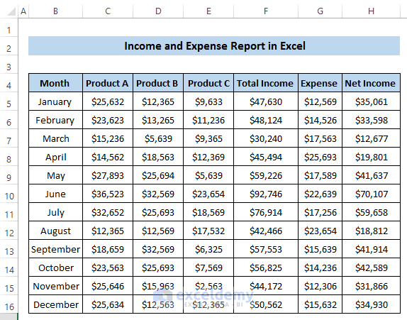
Lastly, we’ll create a monthly income and expense report for a year.
Step 1 – Import Dataset
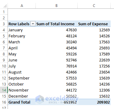
We’ll use the following dataset containing income and expenses for the same company as above, but for individual months instead of days.
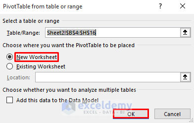
Step 2 – Create Pivot Table
- Select the whole dataset by selecting any cell and pressing Ctrl+A.
- Go to the Insert tab on the ribbon.
- Select PivotTable.
The PivotTable from table or range dialog box will pop up.
- The Table/Range should be pre-filled with the selected range.
- ChooseNew Worksheet to place the PivotTable in a new worksheet.
- Click on OK.
- Go to the worksheet where the PivotTable is located.
- In the PivotTable Fields section, select Month, Total Income, and Expense.
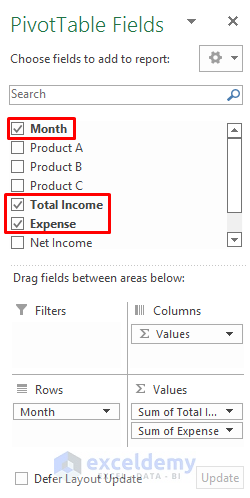
The following table with the selected column headers from PivotTable Fields will appear.
Step 3 – Insert Monthly Income and Expense Report Chart
Now we plot the charts.
- Select any cell in the Pivot Table.
- Go to the Insert tab on the ribbon.
- From the Chart group, select Recommended Charts.
The Insert Chart dialog box will appear.
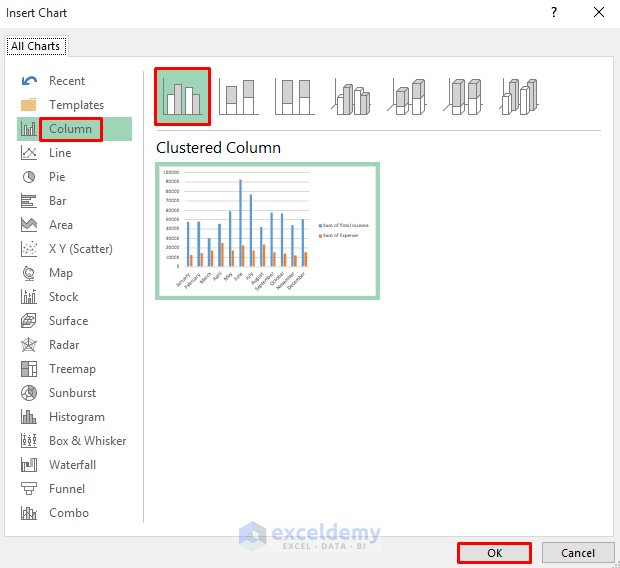
- Select the Column chart from the All Charts section.
- Select a chart, for example the first column chart.
- Click on OK.
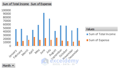
We have our desired chart.
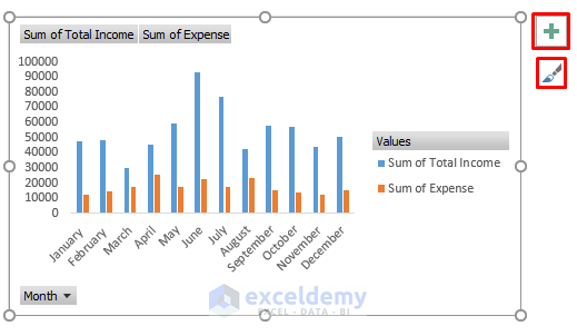
- Modify the column chart by using the Brush and Plus sign.
- The Brush sign can change the chart style.
- The Plus sign can change the chart elements.
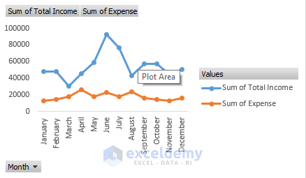
To plot a Line chart:
- Select any cell in the Pivot Table.
- From the Charts group, select Recommended Charts.
The Insert Chart dialog box will appear.
- Select the Line chart from the All Charts section.
- Select a chart, for example the fourth Line chart.
- Click on OK.
We have our desired
- Line
chart.
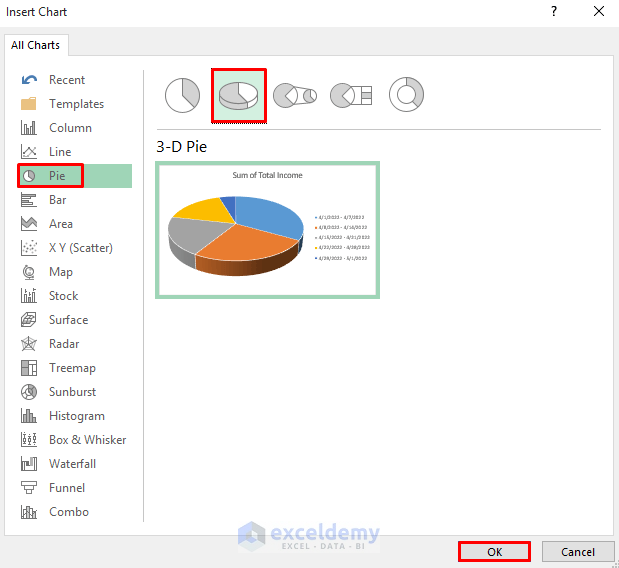
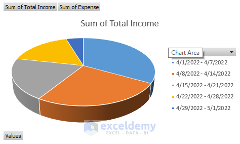
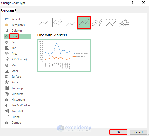
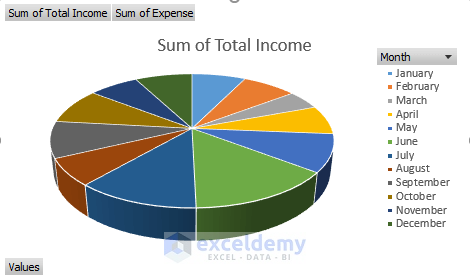
For a Pie chart:
- Go to the Insert tab on the ribbon.
- From the Charts group, select Recommended Charts.
The Insert Chart dialog box will appear.
- Select the Pie chart from the All Charts section.
- Select a chart, for example the second Pie chart.
- Click on OK.
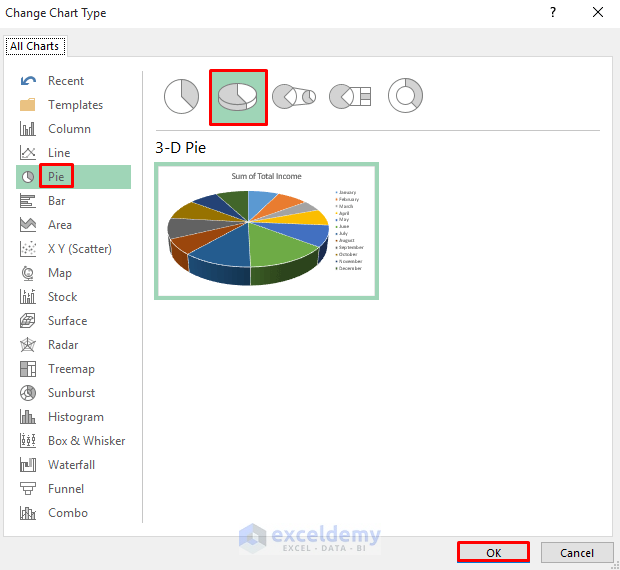
We have our desired Pie chart.
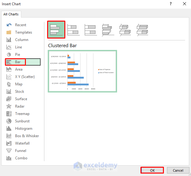
Finally, we’ll create a Bar chart.
- Go to the Recommended Charts option like for the previous charts.
The Insert Chart dialog box will appear.
- Select the Bar chart from the All Charts section.
- Select a chart, for example the first Bar chart.
- Click on OK.
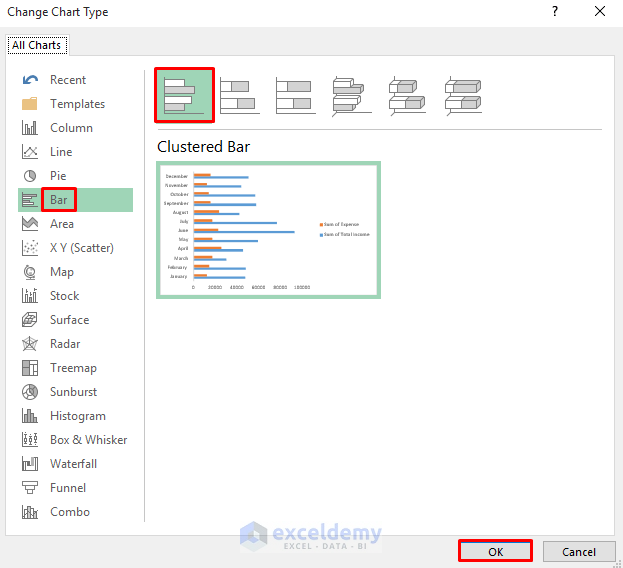
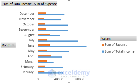
A Bar chart like the following will be created.
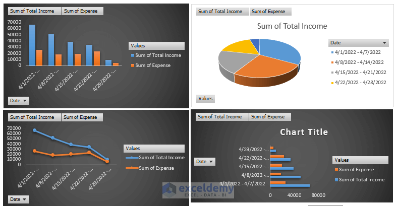
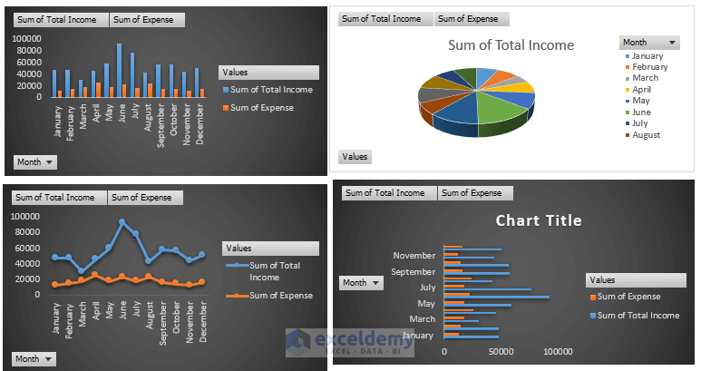
Step 4 – Create Final Daily Income and Expense Report
Copy and paste the charts into a new worksheet presented in the following way:
Related Articles
- How to Create an Expense Report in Excel
- How to Make Production Report in Excel
- How to Make Daily Production Report in Excel
- How to Make a Monthly Expense Report in Excel
- How to Make Daily Activity Report in Excel
- How to Make Monthly Report in Excel
<< Go Back to Report in Excel | Learn Excel
Get FREE Advanced Excel Exercises with Solutions!
