How to Make Report Card in Excel (Download Free Template)

Essential Parts of a Report Card

Part 1 – Student Information

This section includes student information like student IDs, names, classes, sections, institution information, term information, grading system, etc.

Part 2 – Mark Sheet

This section lists all marks and grades for each subject and term.

Part 3 – Term-Wise Report Card

In this section, we have a report card of an individual student for a single term.

Part 4 – Cumulative Report Card

This section sums the term-based report cards into a single sheet.

How to Make a Report Card in Excel (With Easy Steps)

In our practice workbook, we have made a report card in Excel for 10 students in class IX. We’ll prepare 4 worksheets in our dataset for the four essential parts of a report card.

Steps to Make a Report Card in Excel

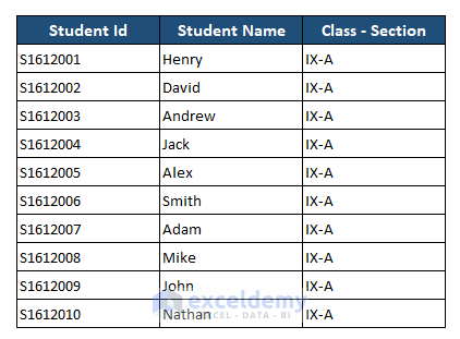
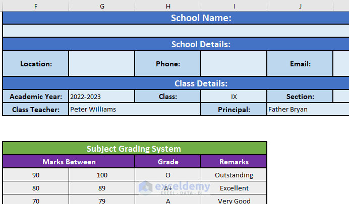
Step 1 – Create a Basic Information Sheet

Prepare a sheet containing student IDs, names, classes, sections, institution’s name, location, principal, class teacher’s name, grading system, etc.

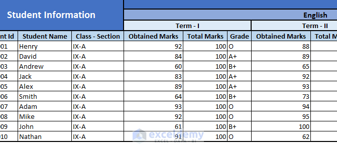
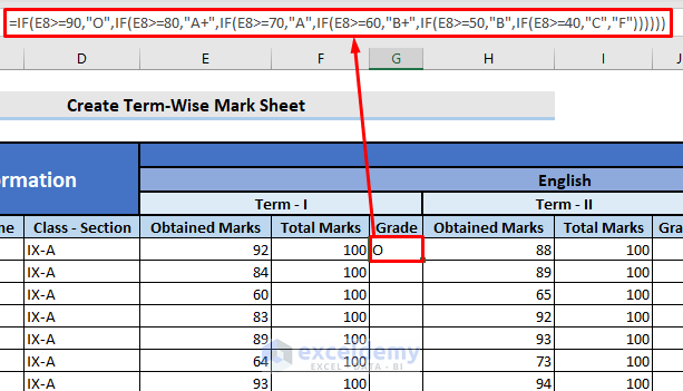
Step 2 – Create the Term-Wise Students’ Mark Sheet

Record the IDs and names of the students and marks obtained in each subject at each term.
From the marks, you need to record the grades of the students in each subject too. Use the following formula in G8.

=IF(E8>=90,"O",IF(E8>=80,"A+",IF(E8>=70,"A",IF(E8>=60,"B+",IF(E8>=50,"B",IF(E8>=40,"C","F"))))))

How Does the Formula Work?

The first IF function will check if Cell E8 is greater than or equal to 90, If it is True it will return O otherwise it will go to the next IF function.
The next IF function will check if Cell E8 is greater than or equal to 80 it will return A+ or else it will move on to the next IF function.
This pattern is continued through each subsequent IF statement, checking if the value in Cell E8 is greater than or equal to 70, 60, 50, and 40 and returns A, B+, B, and C respectively.
If none of the conditions are True, it will return F.

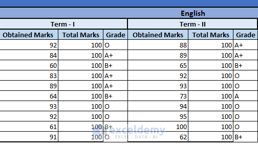
Drag the fill handle and copy the formula for other students.

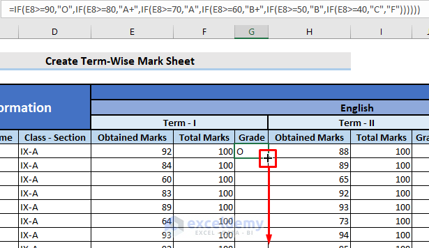
Copy the formula for other subjects and terms.

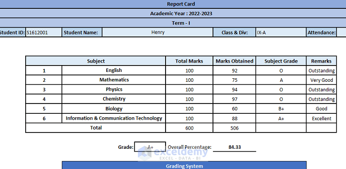
Step 3 – Create a Term-Wise Report Card

Put the fields for the basic pieces of information, such as the student’s ID, name, section, attendance, term number, etc., at the top of the report card.
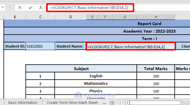
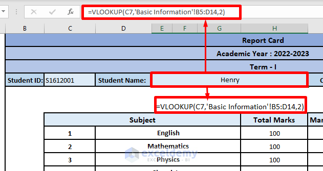
Click on the E7 cell for the name of the student.
Insert the following formula:

=VLOOKUP(C7,'Basic Information'!B5:D14,2)

How Does the Formula Work?

In the VLOOKUP function, we inserted Cell C7 as loopup_value, cell range B5:D14 of Basic Information named worksheet as table_array, and 2 as column_index_num to find the value of Cell C7 from the given cell range and return data from the 2nd column of that range.

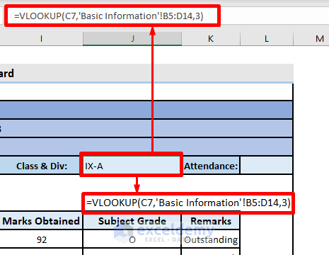
You can also automate the student’s class and section number using the same formula and following the same process. At the col_index_num argument, put 3 since the class and the section are in the third column of our selected range.

From the Term Wise Mark Sheet, record the marks of the student for the following term in each subject.
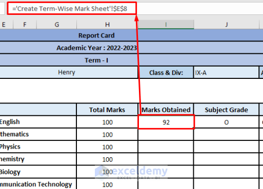
Click on the cell of the Report Card where you want to record the mark of the student.
Put an equal sign(=).
Click on the cell from the Term-Wise Mark Sheet where the mark of the student of that subject was recorded.
Press the Enter button.

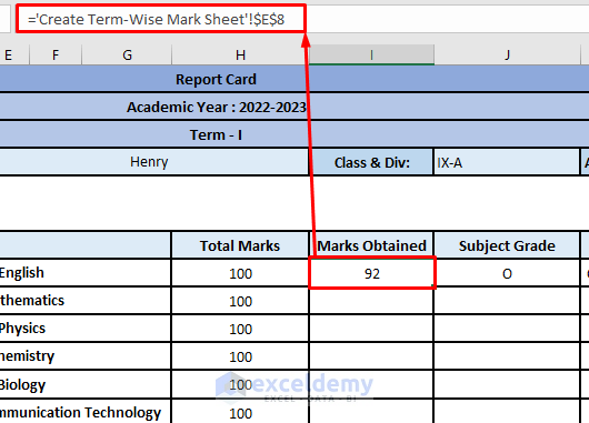
Repeat the process to fill up all the marks obtained cells by referencing them from the Term-Wise Mark Sheet properly.
Record the grade of the students in each subject by using nested IFs from Step 2.
Use the VLOOKUP function again to extract remarks. The lookup value will be the achieved grade of the student. In the Basic Information sheet, there is a column for Remarks according to their Grades. Put the column index number in the formula according to your selection. Write FALSE for Exact match at the last argument.

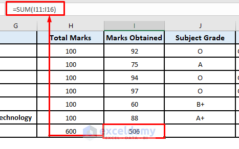
You can find the total marks obtained using the SUM function. Select the cell for the sum.
Write =SUM(.
Select the cell range you want to sum and close the parenthesis.

Use the following formula to get the overall marks percentage.

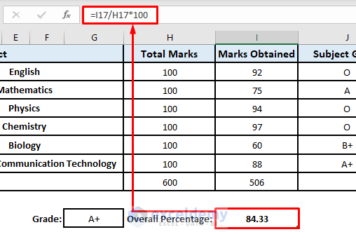
Get the overall grade of the student following the grading system. You can use the nested IF conditions like in Step 2.

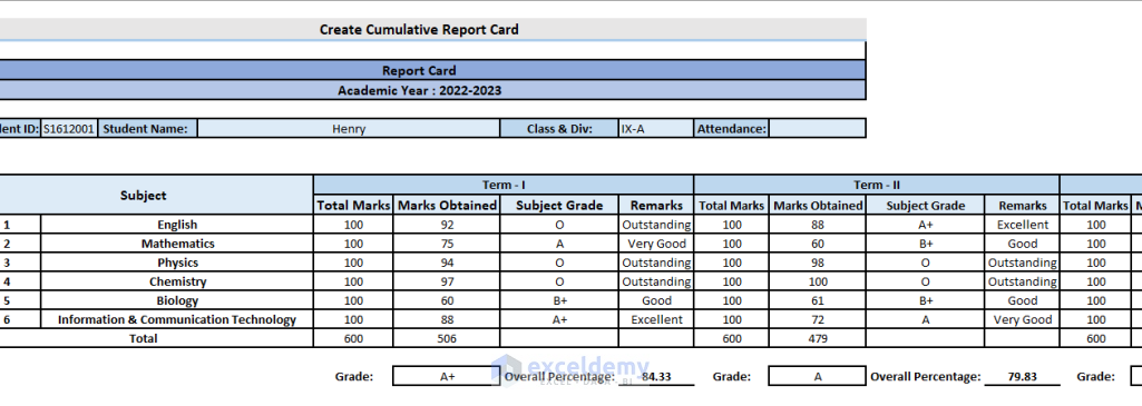
Step 4 – Create Cumulative Report Card

Create the cumulative report card for each student. All term mark sheets will be combined into a single report card.

Things to Remember

When using the VLOOKUP function, you can only look up your values through the columns.
When selecting the table array for VLOOKUP, keep the lookup value column as the first column in your selection. The return value column index number will be put according to this serial.
If you look up numbered values, the range_lookup argument is not as important. But, if you look up text values, put the range_lookup argument as FALSE if you want an exact match always.

Download the Free Report Card Template

Report Card Template.xlsx

<< Go Back to Report in Excel | Learn Excel

Get FREE Advanced Excel Exercises with Solutions!

6 Comments

Elton Feb 12, 2023 at 10:43 AM

I have found this article very helpful,but it could have been nice if you had created a pdf file for such information for us to read properly.
- Reply
  Shamima Feb 13, 2023 at 3:41 PM
  
  Hi, Elton!
  
  Thanks for your appreciation. We will try to launch pdf files.
  
  Regards
  ExcelDemy
Elly Apr 9, 2023 at 1:39 PM

The article is wonderful but please elaborate more on the functions used for proper understanding. Thanks
- Reply
  Shamima Sultana Apr 10, 2023 at 2:18 AM
  
  Dear Elly,
  
  Thanks for your appreciation. We re-explained our formulas to make them more understandable. If you find any difficulty now, let us know in the comment section below.
  
  Regards
  ExcelDemy
Femi Aug 11, 2024 at 9:07 AM

This is great. My question is how do print other students results apart from the first name on the list
- Reply
  Shamima Sultana Aug 12, 2024 at 11:29 AM
  
  Hello Femi,
  
  Thanks for your appreciation. You will need to update the report card based on the student ID then you will be able to print the results for all names of the list.
  While changing the name please update marks of each student.
  
  Regards
  ExcelDemy