How to Make MIS Report in Excel for Accounts (With Quick Steps)

Sometimes it becomes a necessity for us to show our data in an MIS report. This report provides us with lots of flexibility to visualize the changing pattern of our dataset. In this article, we will show you how to make an MIS report in Excel for accounts. If you are interested to know about it, download the practice workbook and follow us.

What Is MIS Report?

MIS stands for Management Information System. MIS is a summarized report to show the filtered data of a vast dataset. This type of report is widely used in our regular professional life to providing the data to the higher authority.

Classifications of MIS Report

According to a person’s requirement, an MIS report can be classified into several types:

• Sales Report
• MIS Report in Accounts
• Budget Report
• Production Report
• Cash Flow Statement Report
• Funds Statement Report
• Profit Report
• Income Statement Report
• Abnormal Losses Report
• Costing Report
• HR Report
• Inventory Report
• Statistical Publication Report
• Orders in Hand Report
• Report on Ideal Time
• Machine Utilisation Report
• Summary Report
• Trend Report
• Exception Report

Advantages

MIS report provides us considerable advantages in our daily professional life.

• MIS report helps in data management
• To define the data trend
• Set up the organization’s goal
• Identifying the problems
• Increasing and improving the efficiency of a company
• Reduced the production costs & errors

How to Make MIS Report in Excel for Accounts (With Quick Steps)

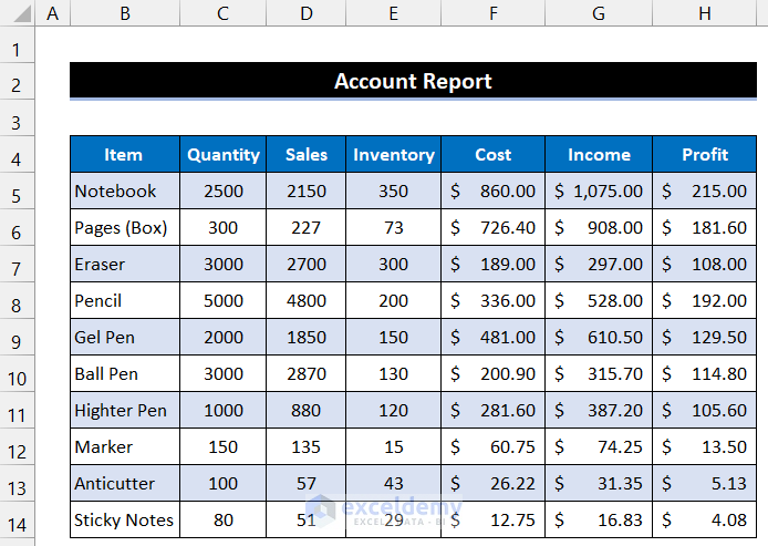
For creating the MIS report, we consider a dataset of a stationery shop’s account report for a month. In our dataset, we take a list of 10 stationery products in column B. Their quantity is in column C, the sales amount of that month is in column D, and the remaining inventory is in column E. The cost of the shop owner, income, and profit are in columns F, G, and H respectively. Thus, we can say our dataset is in the range of cells B5:H14.

Step 1: Import Your Dataset

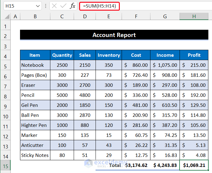
Here, we are going to input our dataset into Microsoft Excel. Besides it, you can import it from other types of data files. Use the SUM function to get the summation of the Cost, Income, and Profit columns.

• To sum the Profit write down the following formula in cell H15.

• Now, follow the same process for F15 and G15 to get the sum of Cost and Income.

Step 2: Create Pivot Table

In this step, we will create a Pivot Table of our dataset. We want to include the Quantity, Sales, and Inventory column in our pivot table.

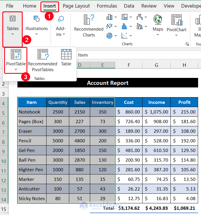
• First of all, select the entire range of cells B4:E14.

• Then, in the Insert tab, select the PivotTable from the Tables group.

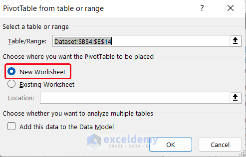
• As a result, a small dialog box called PivotTable from table or range will appear.
• Make sure to check the New Worksheet option to preserve your original dataset.
• Finally, click OK.

• You will see a new sheet created entitled Sheet in the Sheet Name Bar.
• In that sheet, you will see a side window titled Pivot Table Field. You will also see the columns’ names here.

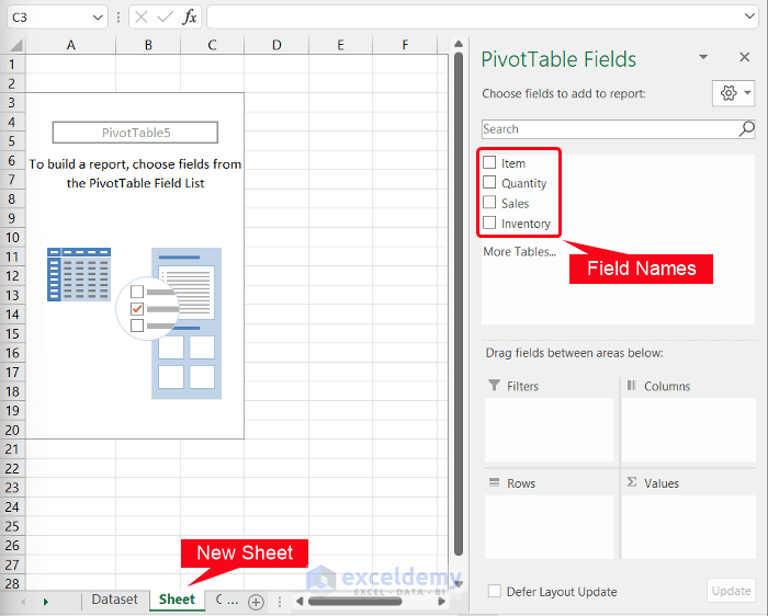
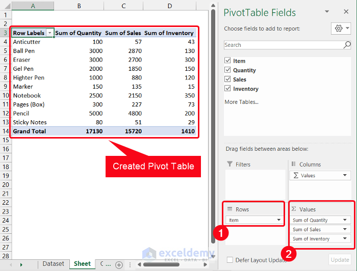
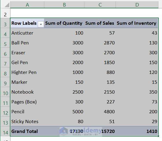
• Now, drag the field name into the 4 boxes below the title Drag fields between areas below according to your desire. We keep the Item in the Rows and the other three columns in the Values.
• You will see that when you start to input the field name into that four boxes, they will insert into the pivot table one by one.
• Finally, click the Close button on the right corner of that side window to close.

Step 3: Insert Charts for Pivot Fields

In this step, we will insert four different types of charts to show our data pattern. Among them, two will be Column charts, one will be a Bar chart, and the last one will be a Pie chart.

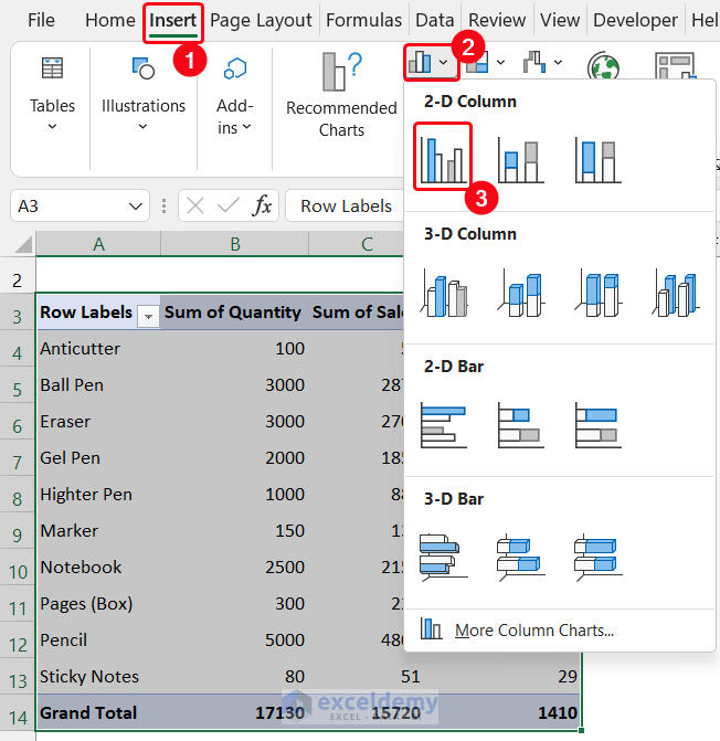
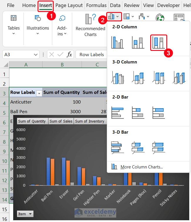
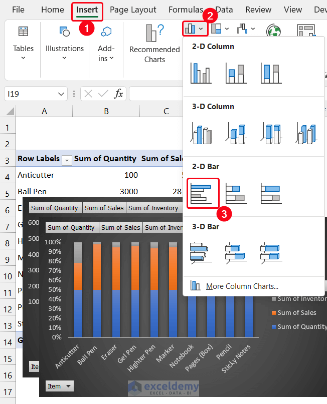
• First, select the entire range of cells A3:D14.

• Now, select the drop-down arrow of the Column or Bar Chart from the Charts group.
• Then, select the Clustered Column option from the 2-D Column section.

• The chart will appear in front of you. After that, click on the Chart Element icon and check the elements you want to keep. In this case, we checked only the Axes and Data Table element for our convenience.

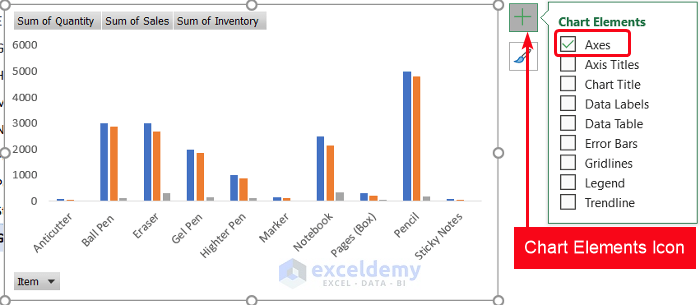
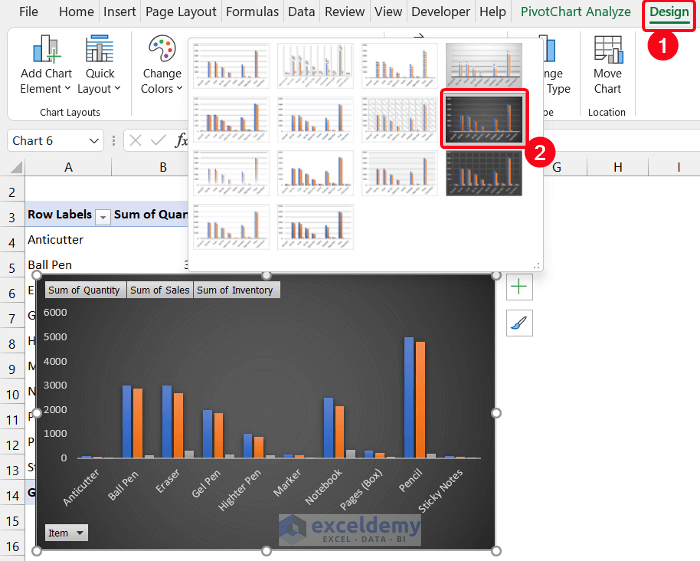
• You can also modify your chart style and texts from the Design and Format tabs.
• We choose Style 8 for our chart. For that, select the Style 8 option from the Chart Styles group.
• Then, use the Resize icon at the edge of the chart for better visualization.

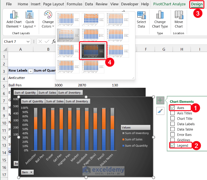
• Now, again select the whole pivot table and from the Charts group, insert the 100% Stacked Column from the drop-down arrow of Column or Bar Chart.

• Next, click on the Chart Element icon and keep the Axes and Legend in this chart. Besides it, we keep the same chart style as the previous chart.

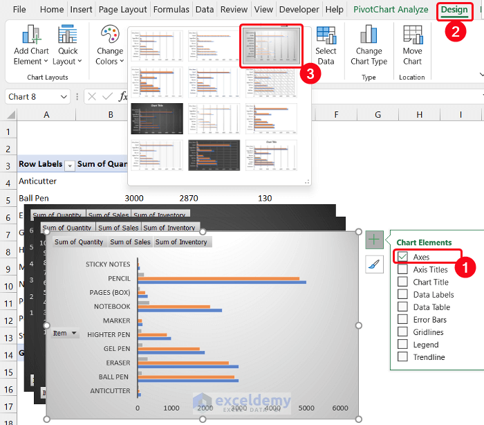
• Similarly, for the Bar chart, follow the same process, and in the drop-down arrow of Columns or Bar Chart, select the Clustered Bar option from the 2-D Bar section.

• Now, modify the number of elements and the chart style according to your desire. We choose Style 3 and only the Axes element in this chart.

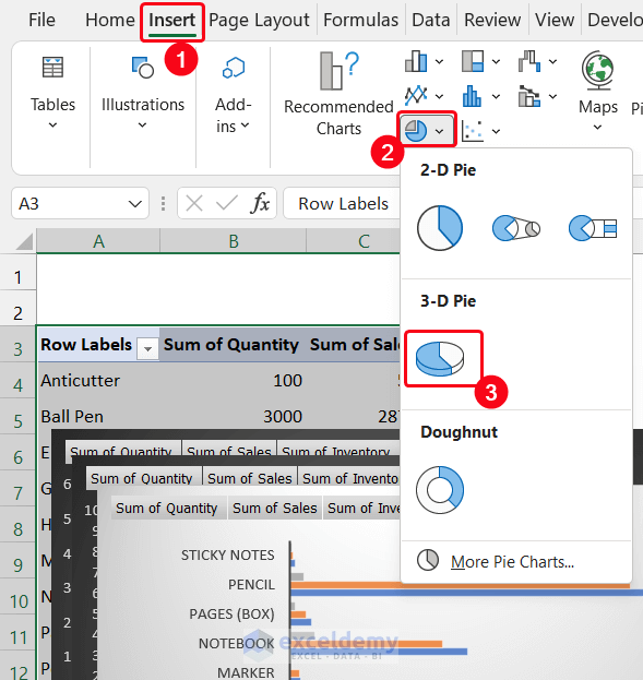
• Finally, for the Pie chart, select the entire range of cells A3:D14 and select the drop-down arrow of the Insert Pie or Doughnut Chart option.
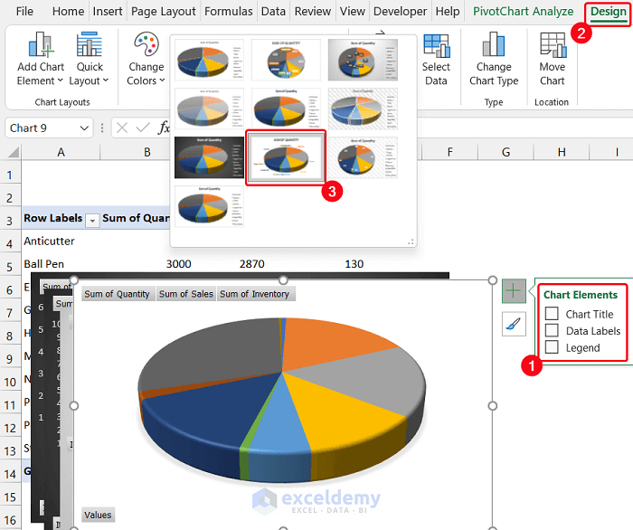
• Now, select the 3-D Pie option.

• Then, adjust the chart style. We chose Style 8 for our chart and eliminated all the chart elements.

Step 4: Insert Slicer

Here, we are going to insert the Slicer into our Excel spreadsheet. The Slicer provides us with lots of flexibility while we filter our data.

• To insert the Slicer, go to the Pivot Chart Analyze tab.
• Now, select the Inset Slicer option from the Filter group.

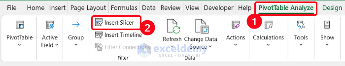
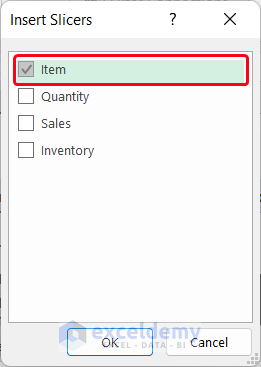
• A small dialog box entitled Insert Slicer will appear.
• Then, check the field you want in the Slicer. For our dataset, we only choose the Item field.
• Click OK to close the dialog box.

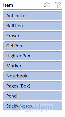
• You will get the Slicer titled as Item and contain all the values of the Item column.
• After that, use the Resize icon at the edge of the Slicer to show all the values.

Step 5: Generate MIS Report

Now, we will show our charts in a separate sheet as a report. If you look at this sheet all of the charts are placed one upon another and we are not able to visualize them.

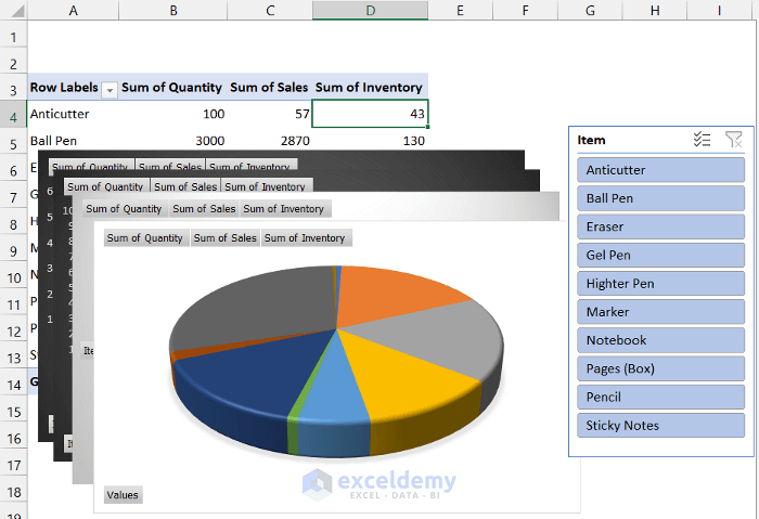
• To create the report, create a new sheet and set the name of that sheet. We set the sheet name as Report.
• Now, select a chart and from the PivotChart Analyze tab, select the Move Chart option from the Action group.

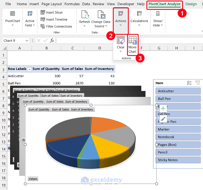
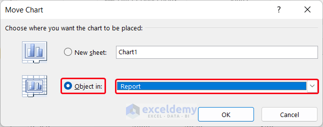
• As a result, the Move Chart dialog box will appear in front of you.
• Then, check the Object in option, and from the drop-down arrow of that box choose the Report sheet.
• Finally, click OK and you will find the chart moved into that sheet.

• Besides it, you can select a chart and press ‘Ctrl+C’ to copy the chart.
• Then, go to the Report sheet and press ‘Ctrl+V’ to paste. It will make a copy of your chart.
• Now, follow the same process for the rest of the elements.
• After that, rearrange them in the sheet to get a perfect visualization of all the charts and the Item Slicer.

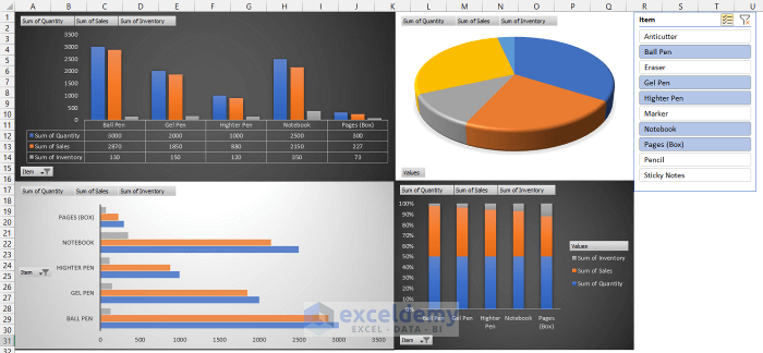
• You will get your MIS report ready to use.

Finally, we can say that our working procedure worked perfectly and we are able to make an MIS report in Excel for accounts.

Download Practice Workbook

Download this practice workbook for practice while you are reading this article.

Conclusion

That’s the end of this article. I hope that this article will be helpful for you, and you will be able to make an MIS report in Excel for accounts. Please share any further queries or recommendations with us in the comments section below if you have any further questions or recommendations.

Related Articles

• How to Prepare MIS Report in Excel
• How to Make MIS Report in Excel for Sales
• Create a Report that Displays the Quarterly Sales by Territory
• How to Make Monthly Sales Report in Excel
• How to Make Daily Sales Report in Excel
• How to Make Sales Report in Excel
• Create a Report That Displays Quarterly Sales in Excel

<< Go Back to Report in Excel | Learn Excel