How to Calculate Square Root in Excel (6 Suitable Ways)

In analyzing datasets in Excel, we often need to find the square roots of the numerical data. The square root of any number is nothing but the application of the power ½  on the number. In this article, we will discuss how to square root in Excel in 6 different ways.

How to Square Root in Excel: 6 Suitable Ways

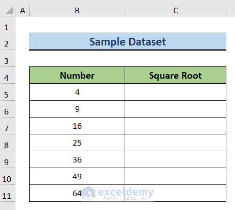
In this article, we will discuss 6 ways to find square roots in Excel. Firstly, we will use the carat operator. Secondly, we will utilize the SQRT function. Thirdly, we will use the POWER function to determine the root. In the next method, we will apply the SERIESSUM function to get the result. Then, we will opt for POWER QUERY to accomplish our task. Finally, we will resort to a simple VBA code to calculate square root in Excel. We will use the following sample dataset to illustrate the methods.

1. Using Carat Operator

The carat operator(^) is the default operator to display the degree of power a number has. In this method, we will use this application of the operator to find the square root of numbers.

Steps:

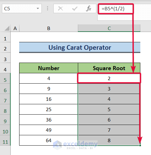
• Firstly, select the C5 cell and write the following formula,

• Here, we assigned the power ½ to the number in the B5 cell.
• Finally, hit Enter.

• Consequently, you will find the square root of the number in the C5 cell.
• In our case, the square root is 2.
• Then, move the cursor down to find the square roots of the rest of the data.

2. Utilizing SQRT Function

The SQRT function is the default function of Excel to find the square root of numbers. In this instance, we will use the function to calculate the square roots.

Steps:

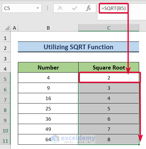
• To begin with, select the C5 cell and write the following formula,

• Then, hit Enter.

• As a result, the C5 cell will contain the value of the number’s square root.
• In this case, the square root is 2.
• After that, find the square roots of the remaining data by lowering the cursor.

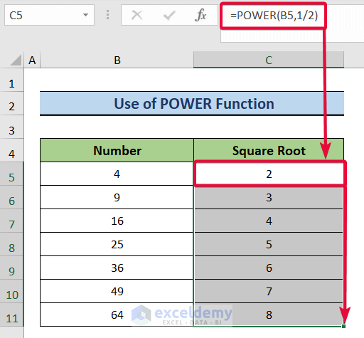
3. Use of POWER Function

The POWER function returns the result of a number raised to a power. In this method, we will use the POWER function to generate a number whose power is raised to a power of ½.

Steps:

• To start with, select the C5 cell and write the following formula,

• Here, we will raise the power of the number in the B5 cell to ½.
• Finally, hit Enter.

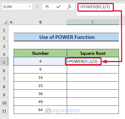
• As a result, the square root of the number will be represented in the C5 cell.
• In this instance, the square root is 2.
• After that, lower the cursor down to find the square roots of the remaining data.

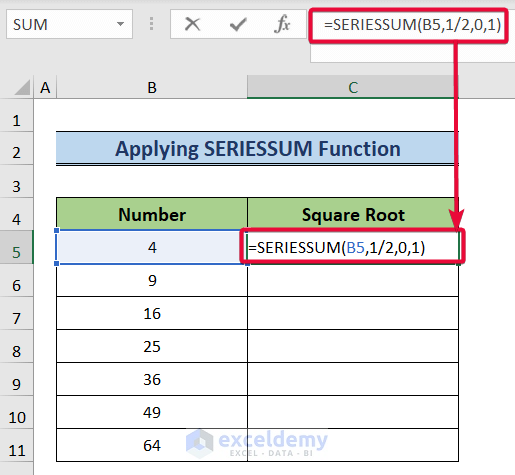
4. Applying SERIESSUM Function

The SERIESSUM function is used to calculate the sum of a power series. In this example, we will use the formula systematically to find the square root of different numbers.

Steps:

• Firstly, select the C5 cell and write the following formula down,

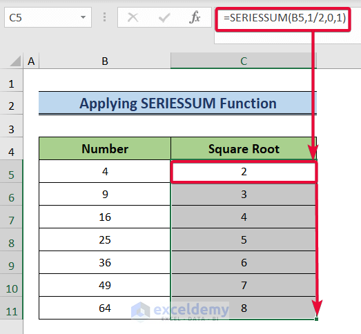
• Here, the first value is the value at which we will evaluate the series.
• In this case, the value is 4.
• The next argument is the starting power of the series.
• In our case, it is ½.
• The subsequent argument is the progression in the series’ power increase.
• In this case, we do not want to increase our series power. Since we do have only one number.
• So, we will set the argument value to zero.
• The final argument is the coefficients of the numbers in the series.
• In this instance, the only number we have is 4 and its coefficient is
• Finally, hit Enter.

• As a result, we will have the square roots of the number.
• Then, move the cursor down to the last data cell to get the square root of all the numbers.

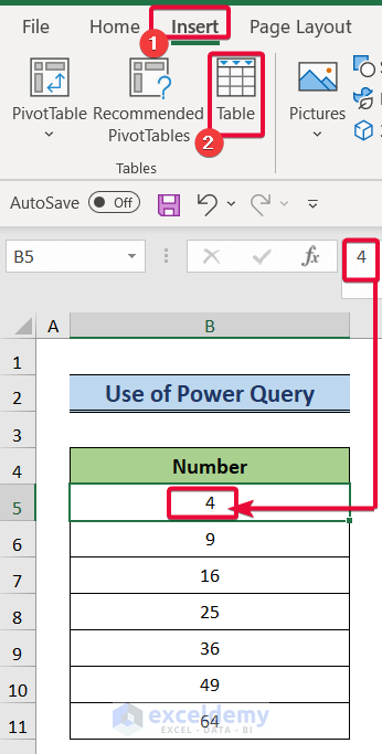
5. Use of Power Query

In this method, we will use Power Query to add a column named “Square Root” beside our existing dataset and then calculate the square root of the numbers.

Steps:

• Firstly, select a data value from a dataset.
• Then, go to the Insert tab in the ribbon.
• From the Insert tab, select the Table option.

• Secondly, in the Create Table prompt, select the entire dataset as table data.
• Then, click OK.
• Consequently, the dataset will be turned into a table from range data.

• After that, choose the Data tab from the ribbon.
• Then, select From Table/Range.

• In the Power Query window, first, go to the Add Column toolbar.
• From there select Custom Column.
• As a result, a window will pop up.

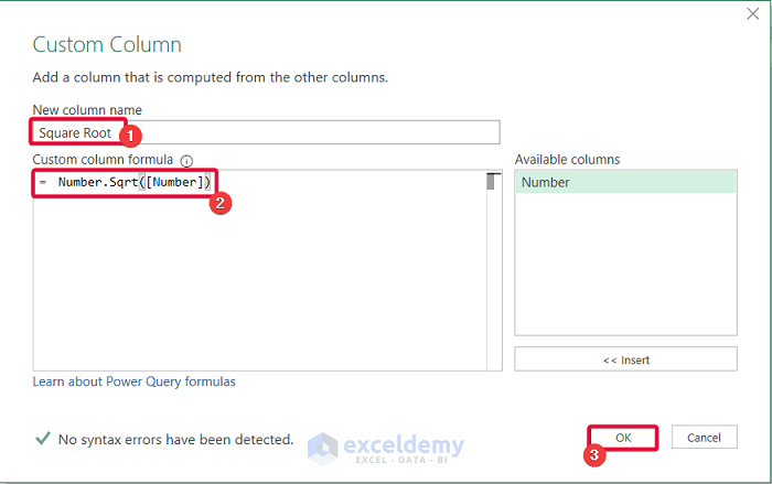
• In the Custom Column window, first, name the new column in the New column name box.
• In this instance, the name is Square Root.
• Then, in the Custom column formula write down the following formula,

• The formula applies the SQRT function to all the numbers in the Number column.
• Finally, click OK.

• After that, go to the Home tab of the Power Query window.
• From there, select the Close & Load tab.
• Finally, from the drop-down option select the Close & Load command.

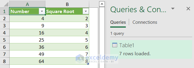
• Consequently, we will have the square roots of the numbers in a new window in a new column named “Square Root”.

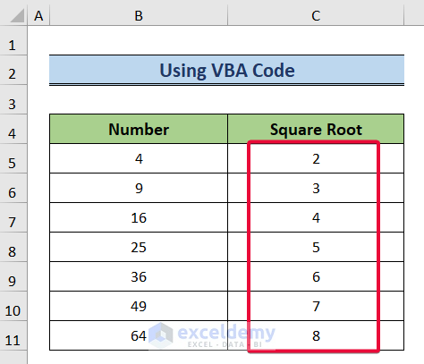
6. Using VBA Code

In the final method, we will resort to a VBA code to calculate square root in Excel. The code applies the Sqrt function to each of the numbers on the list.

Steps:

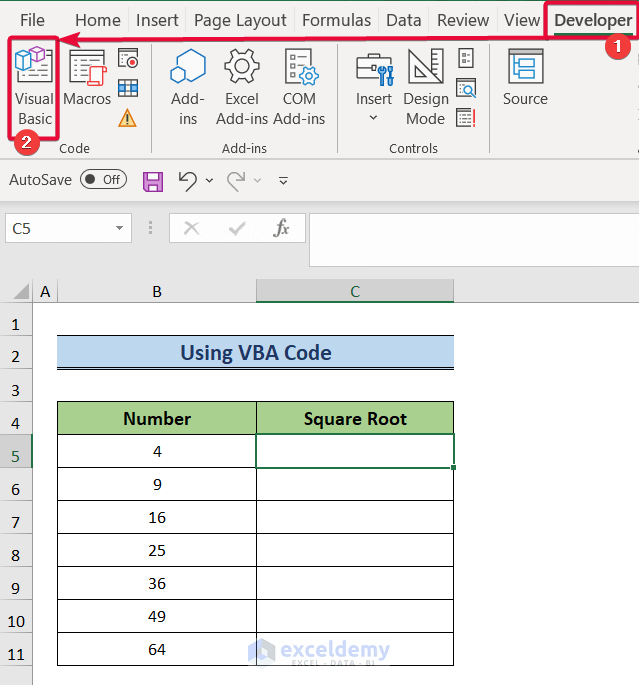
• Firstly, go to the Developer tab in the ribbon.
• From there, select the Visual Basic tab.
• Consequently, the Visual Basic window will be opened.

• After that, in the Visual Basic tab, click on Insert.
• Then, select the Module option.
• Consequently, a coding module will appear.

• In the coding module, write down the following code.
• Then, save the code.

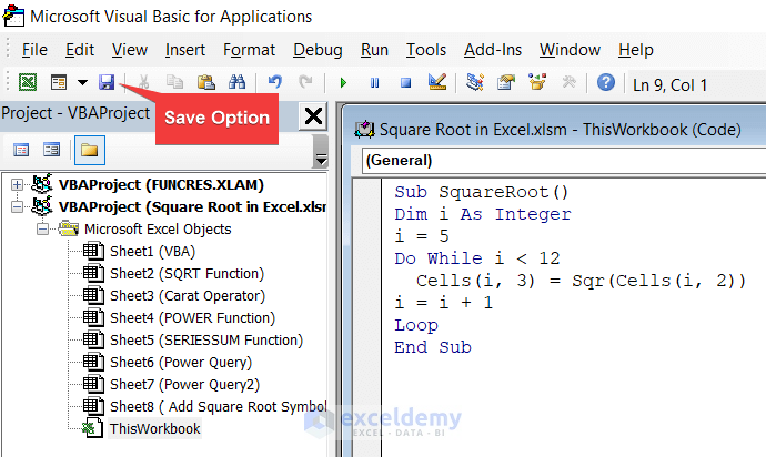
Sub SquareRoot()
Dim i As Integer
i = 5
Do While i < 12
  Cells(i, 3) = Sqr(Cells(i, 2))
i = i + 1
Loop
End Sub

• Finally, go to the Run tab and click on it.
• From the drop-down option, select the Run command to run the code.

• Consequently, you will be able to calculate the square roots of the numbers.

Read More: How to Do Cube Root in Excel

How to Insert Square Root Symbol in Excel

In this additional method, we will add the square root symbol in our Excel sheet by using the UNICHAR function. The UNICHAR function displays a certain character in a cell if we pass the specific number assigned to that character as the argument of the function.

Steps:

• Firstly, select the C5 cell and write down the following formula,

• Here, we will pass the number 8730 as the argument of the UNICHAR function.
• 8730 is the number associated with the square root character.
• The ampersand sign will be used to concatenate the square root symbol with the number in the B5 cell.
• Finally, hit Enter.

• Consequently, you will find that the square root character is added to the number.
• Now, lower the cursor to the last cell of the dataset to add the character to all the numbers.

Read More: How to Find Nth Root in Excel

Download Practice Workbook

You can download the practice workbook from here.

Conclusion

Finding the square root of a number is an essential operation in any data analysis. After going through this article, the readers will have a clear understanding of the ways to calculate the square root of a number in Excel.