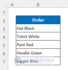
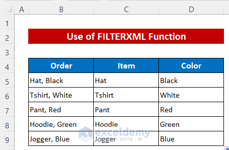
To showcase the methods, we will use a simple dataset listing some items of clothing and their corresponding colors, and apply a formula to split each item into its Name and Color.
Method 1- Use LEFT and FIND Functions to Split Text in Excel
This method will be used to split the Name from the text.
The SEARCH function can be used interchangeably with the FIND function.
Steps:
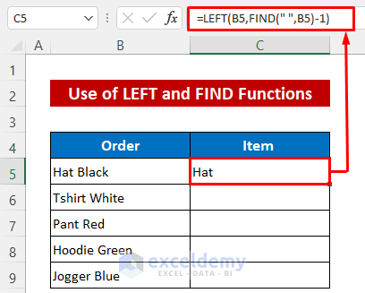
- Enter the following formula in Cell C5–
=LEFT(B5,FIND(" ",B5)-1)- Press Enter to get the result.
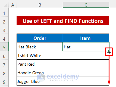
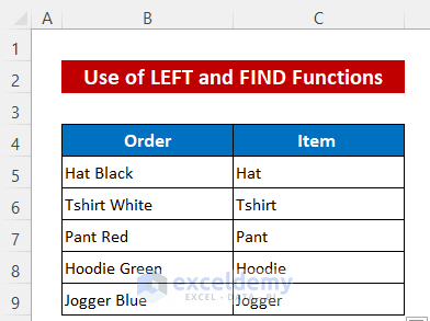
- Drag down the Fill Handle icon to copy the formula to the other cells in the series.
- FIND(” “,B5)-1
The FIND function returns the position of the text specified in the first parameter (“ “) within the text specified in the second parameter (cell B5). We subtract 1 from the result, to skip the searched text (“ “). The function returns 3.
- LEFT(B5,FIND(” “,B5)-1)
The LEFT function returns only the first x characters of the first parameter (cell B5), where x is the number specified in the second parameter (3), ie our formula seeks the first 3 characters of cell B5, and returns “Hat”
Read More: How to Split Text by Space with Formula in Excel
Method 2 – Use RIGHT, LEN, and FIND Functions to Split Text in Excel
This method will be used to split the Color from the text.
The SEARCH function can also be used interchangeably with the FIND function here.
Steps:
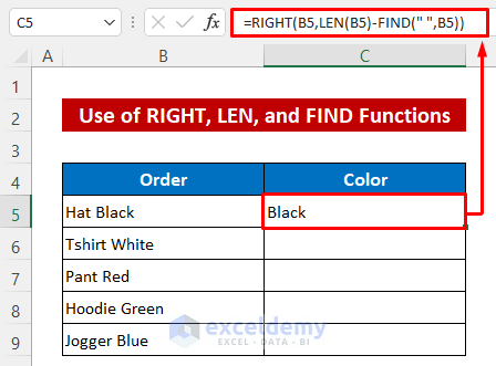
- Enter the following formula in Cell C5 –
=RIGHT(B5,LEN(B5)-FIND(" ",B5))- Press Enter to get the result.
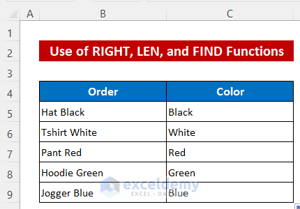
- As in Method 1, use the Fill Handle tool to copy the formula to the rest of the series.
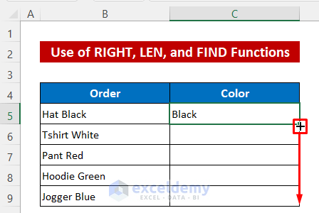
The output should look as follows:
- FIND(” “,B5)
The FIND function (described in Method 1 above) returns 4. - LEN(B5)-FIND(” “,B5)
The LEN function returns the total number of characters in the specified text (Cell B5). We subtract the output of the FIND function from the total length to return the number of characters after the “ “, ie 5. - RIGHT(B5,LEN(B5)-FIND(” “,B5))
The RIGHT function returns only the string in the first parameter (cell B5) remaining after removing the first x characters, where x is the number specified in the second parameter (4), ie our formula seeks the string to the right of the first 4 characters of cell B5. The formula returns
“Black”
Read More: How to Split String by Length in Excel
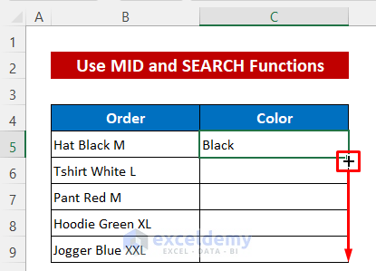
Method 3 – Insert MID and SEARCH Functions in Excel to Split Text
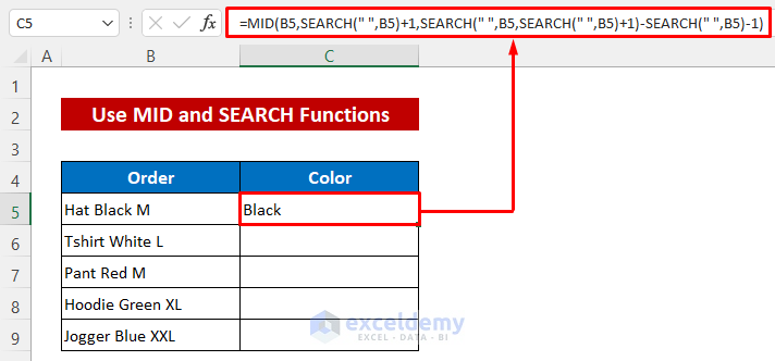
This method can be used to split text from any position in the middle of a string.
To demonstrate, our dataset has been modified to add a size after the color, so the color is now in the middle position. Our function will return just the color.
Steps:
- In Cell C5, enter the following formula-
=MID(B5,SEARCH(" ",B5)+1,SEARCH(" ",B5,SEARCH(" ",B5)+1)-SEARCH(" ",B5)-1)- Press Enter to get the result.
- As with previous Methods, copy the formula using the Fill Handle tool.
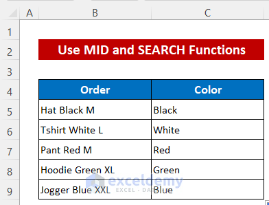
The output should look like this:
Formula Breakdown
- SEARCH(” “,B5,SEARCH(” “,B5)+1)-SEARCH(” “,B5)-1
Returns the number of characters to retain, namely
5
- SEARCH(” “,B5)+1
Returns the starting position for the MID function, ie the position of the first space character in cell B5, plus 1 character to skip past it. The function returns
5
- MID(B5,SEARCH(” “,B5)+1,SEARCH(” “,B5,SEARCH(” “,B5)+1)-SEARCH(” “,B5)-1)
The MID function retains the string starting from the position specified in parameter 1, and ending after the number of characters specified in parameter 2. The formula returns
“Black”
Read More: How to Split First And Last Name in Excel
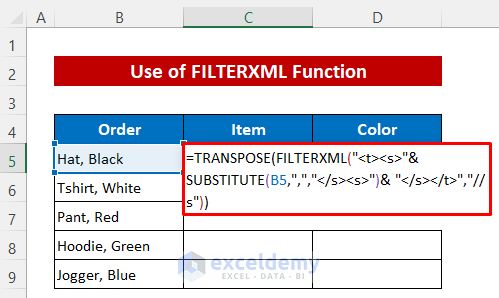
Method 4 – Apply Excel FILTERXML Function to Split Text
Using the FILTERXML function, we can easily split both the name and color at the same time. This method also makes use of the TRANSPOSE and SUBSTITUTE functions.
Steps:
- Enter the following formula in Cell C5:
=TRANSPOSE(FILTERXML("<t><s>"&SUBSTITUTE(B5,",","</s><s>")& "</s></t>","//s"))- Use the Fill Handle tool to copy the formula to the other cells in the series.
- Use the Fill Handle tool to copy the formula to the other cells in the series.
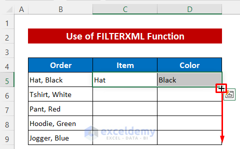
Result: all the items and colors have been split into their own columns.
Formula Breakdown
- FILTERXML(“<t><s>”&SUBSTITUTE(B5,”,”,”</s><s>”)& “</s></t>”,”//s”)
This function returns the text strings as XML strings, by converting the delimiter letters into XML tags. It returns –
{“Hat”,”Black”} - TRANSPOSE(FILTERXML(“<t><s>”&SUBSTITUTE(B5,”,”,”</s><s>”)& “</s></t>”,”//s”))
The TRANSPOSE function transposes the output from vertically to horizontally. It returns –
{“Hat”,”Black”}
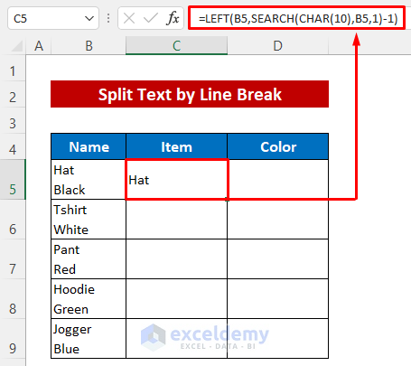
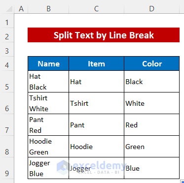
Method 5 – Use a Combined Formula to Split Text with Line Breaks.
Text with line breaks can also be split easily using a formula. To demonstrate this method, line breaks have been added to our dataset.
Steps:
To split the item name:
- Enter the following formula in Cell C5 –
=LEFT(B5,SEARCH(CHAR(10),B5,1)-1)- Press Enter to get the result.
Formula Breakdown
- Refer to Method 1 to understand how the formula works. Here, we simply replaced the space character with CHAR(10), which is the ASCII code for the Line Break.
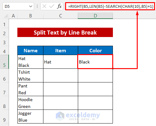
To split the color:
- Enter the following formula in Cell D5 –
=RIGHT(B5,LEN(B5)-SEARCH(CHAR(10),B5)+1)- Press Enter to get the result.
Formula Breakdown
- Refer to Method 2 above to understand how the formula works. We simply replaced the space character with CHAR(10), which is ASCII code for the Line Break.
- As with the other methods, use the Fill handle tool to copy the formula to the other cells in the series.
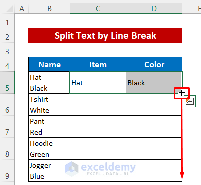
The output should look as follows:
Read More: How to Split Text in Excel by Character
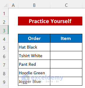
Practice Section
Use the Practice Workbook below to practice the different Methods.
Download Practice Workbook
Related Articles
- How to Split Text in Excel into Multiple Rows
- Split Text after a Certain Word in Excel
- How to Separate Two Words in Excel
- Split String by Character in Excel
- How to Split Text by Number of Characters in Excel
<< Go Back to Splitting Text | Split in Excel | Learn Excel
Get FREE Advanced Excel Exercises with Solutions!
