Method 1 – Using ‘Power Query’
The following dataset has one column showing codes.
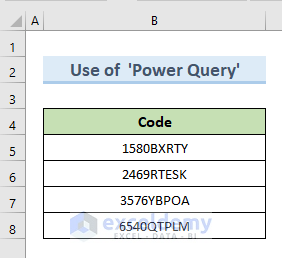
STEPS:
- Select any cell from the data range.
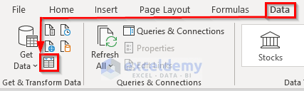
- Go to the Data.
- Select the option ‘From Table/Range’ from the ribbon.
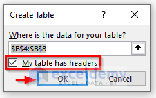
- The above command opens a new dialogue box named ‘Create Table’.
- Check the option ‘My table has headers’ and click on OK.
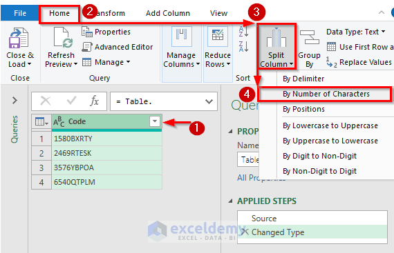
- The new Power Query window opens.
- Select a cell from the data.
- Select Home > Split Column > By Number of Characters
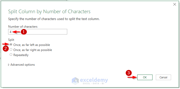
- Enter the value 4 in the ‘Number of characters’ textbox.
- Check the Split option ‘Once, as far left as possible’.
- Click on OK.
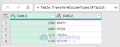
- We get results like the image below.
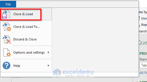
- Go to the File tab and select ‘Close and Load’.
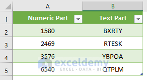
- The following result is in a new worksheet.
NOTE: In this procedure, we have 3 split options:
- Once, as far left as possible: Counts the characters of the first split column from the left and the second split column from the right.
- Once, as far right as possible: Enumerate the characters of the first split column from the right and the second split column from the left.
- Repeatedly: Split the original column into multiple columns depending on the number of characters. If the initial column has 20 characters and the number of characters is set to 4, we’ll get 5 new columns, each with 5.
Read More: How to Split Text in Excel by Character
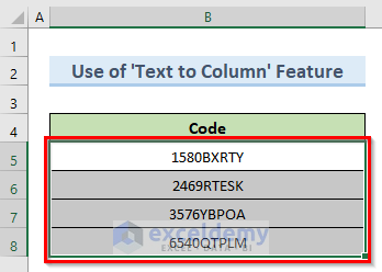
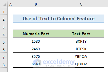
Method 2 – Using the ‘Text to Column’ Feature
STEPS:
- Select a cell range (B5:B8).
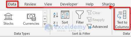
- Go to the Data.
- Select the option ‘Text to Columns’ from the ribbon.
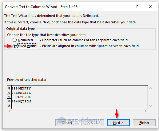
- Select the option Fixed width from the ‘Convert Text to Columns Wizard’ window and click on the Next button.
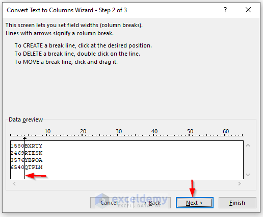
- From the ‘Convert Text to Columns Wizard,’ click on the desired position from where we want to split the data.
- Click on the Next button.
- Select the option General and click on the Finish button.
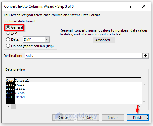
- We get results like the image below.
Read More: How to Split Text in Excel into Multiple Rows
Method 3 – Apply LEFT & FIND Functions
STEPS:
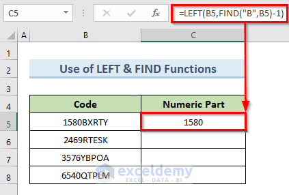
- Select cell C5.
- Enter the following formula in that cell:
=LEFT(B5,FIND("B",B5)-1)- Press Enter.
- In cell C5, we get only the numeric part from the value of cell B5.
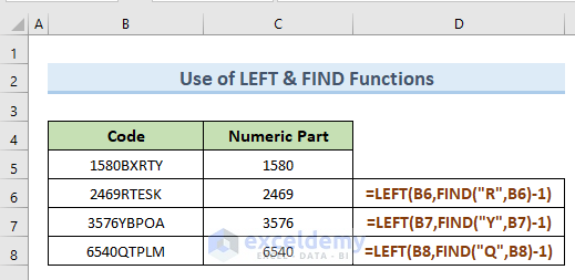
- Enter the corresponding formulas for cells C6, C7, and C8, like the following image.
- We get the values of the numeric part, like the image below.
How Does the Formula Work?
- FIND(“B”,B5): This part returns the position of character B in text string B5. The return value is 5.
- LEFT(B5,FIND(“B”,B5)-1): Here the LEFT function returns characters from the string of cell B5 up to the 5th.
Read More: Split String by Character in Excel
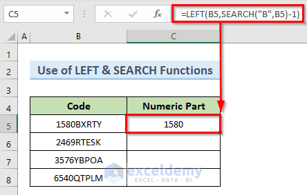
Method 4 – Using LEFT & SEARCH Functions
STEPS:
- Select cell C5.
- Enter the following formula in that cell:
=LEFT(B5,SEARCH("B",B5)-1)- Press Enter.
- In cell C5, we get the numeric part from the value of cell B5.
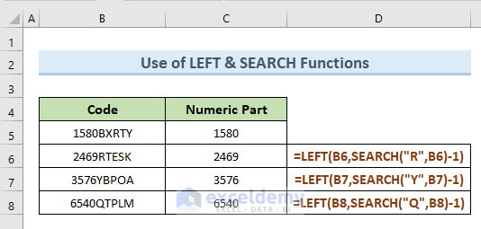
- For cells C6, C7, and C8, enter the relevant formulas, as shown in the image.
- We get results like the image below.
How Does the Formula Work?
- SEARCH(“B”,B5): The position of character B in text string B5 is returned in this section. The value returned is 5.
- LEFT(B5,SEARCH(“B”,B5)-1): Here the LEFT function returns characters from the string of cell B5 up to the 5th character.
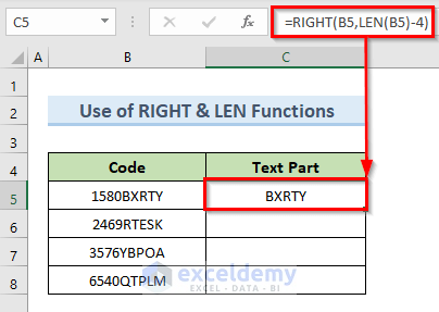
Method 5 – Combining Excel RIGHT and LEN Functions
STEPS:
- Select cell C5.
- Enter the following formula in that cell:
=RIGHT(B5,LEN(B5)-4)- Press Enter.
- In cell C5, we get the value of the text part of cell B5. It returns 5 characters from the right end of the original text string.
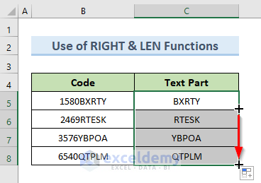
- Drag the Fill Handle tool from cell C5 to C8.
- The result is in the image below.
How Does the Formula Work?
- LEN(B5)-4: This section returns 4 characters less than cell B5’s initial character number.
- RIGHT(B5,LEN(B5)-4): Here the RIGHT function returns the characters from the right end of the string.
Read More: How to Split String by Length in Excel
Method 6 – Using Flash Fill in Excel
STEPS:
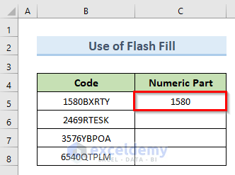
- Select cell C5.
- Enter our desired value in that cell.
- In cell C6, enter the desired value. When we type a digit, we can see that Excel gives us an overview of all our desired outputs.
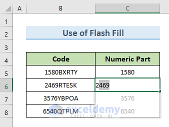
- Press Enter.
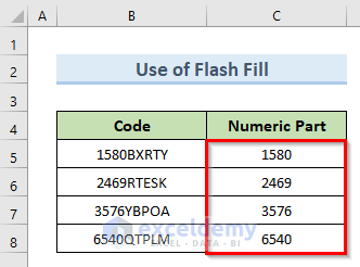
- The result is in the following image.
Read More: How to Split Text in Excel Using Formula
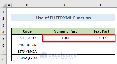
Method 7 – Using Excel FILTERXML Functions
STEPS:
- Select cell C5.
- Enter the following formula in that cell:
=TRANSPOSE(FILTERXML("<s>" &SUBSTITUTE(B5,"-","</s><s>") & "</s>","//s"))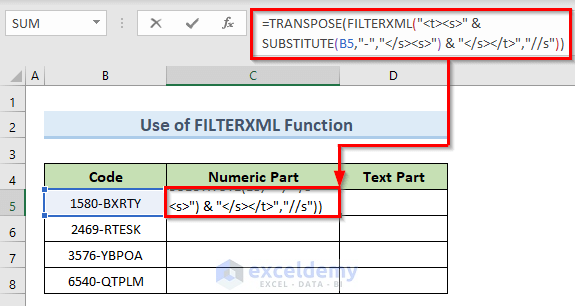
- Press Enter.
- We can see that the numeric part and text part are split by the 5th.
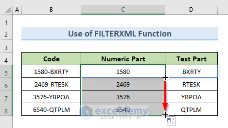
- Drag the Fill Handle tool from cell C5 to C8.
- The result is in the following image.
How Does the Formula Work?
- FILTERXML(“<t><s>” &SUBSTITUTE(B5,”-“,”</s><s>”) & “</s></t>”,”//s”): By replacing the separator characters to XML tags, the text strings will be converted to XML string.
- TRANSPOSE(FILTERXML(“<t><s>” &SUBSTITUTE(B5,”-“,”</s><s>”) & “</s></t>”,”//s”)): Instead of returning the result vertically, the TRANSPOSE function returns it horizontally.
Method 8 – Using MID Function
STEPS:
- Select cell D5.
- Enter the following formula:
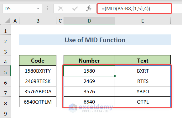
=(MID(B5:B8,{1,5},4))
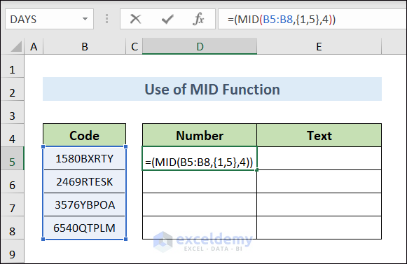
- Press the Enter key.
- We will see the texts and numbers are separated into two different columns.
Download the Practice Workbook
You can download the practice workbook from here.
Related Articles
- Split Text after a Certain Word in Excel
- How to Split Text by Space with Formula in Excel
- Split First And Last Name in Excel
- How to Separate Two Words in Excel
<< Go Back to Splitting Text | Split in Excel | Learn Excel
Get FREE Advanced Excel Exercises with Solutions!

Try this method (the simplest):
=(MID(B5:B8,{1,5},4))
Hello Meni
Thanks for reaching out and sharing your expertise. I have investigated the formula you have shared and found it very powerful. We can easily separate the texts and numbers with this single formula.
Your suggestion proved effective, and We are genuinely grateful for it. Thank you again!
Regards
Lutfor Rahman Shimanto
ExcelDemy Team