Function Type 1 – UPPER, LOWER, and PROPER Functions: Syntax and Arguments
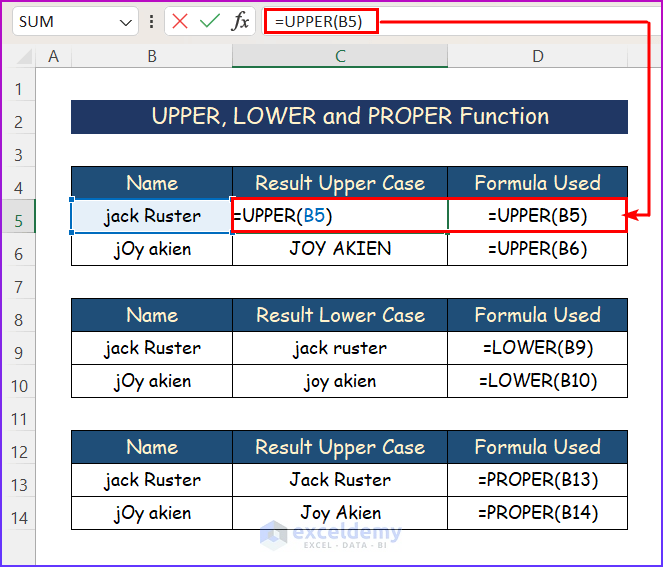
With the UPPER, LOWER or PROPER functions, you can change the case of text to uppercase, lowercase, or proper case. The UPPER function can change a text to all uppercase, The LOWER function can change a text to all lowercase, and the PROPER function will capitalize the first letter of each word.
Syntax:
The syntax of the UPPER function is shown below.
=UPPER(text)
=LOWER(text)=PROPER(text)Arguments:
The syntax has only one argument. It is a required argument or parameter.
| Argument | Required/Optional | Explanation |
|---|---|---|
| text | Required | It is a string of text where all letters have to be converted to upper, lower, or proper cases. |
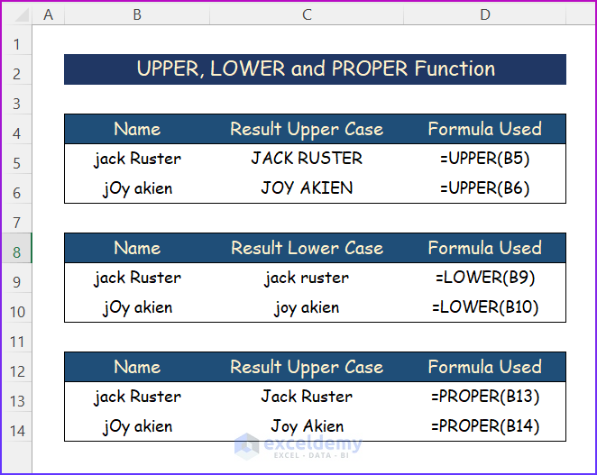
Examples of UPPER, LOWER and PROPER Functions
Steps:
- Click on a cell.
- Enter the following formula to get all letters in upper case.
=UPPER(B5)
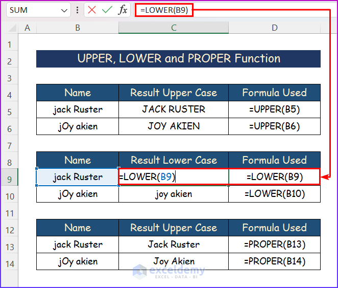
- To get all letters in lowercase, use this formula,
=LOWER(B9)
- To get the proper case, use this formula,
=PROPER(B13)
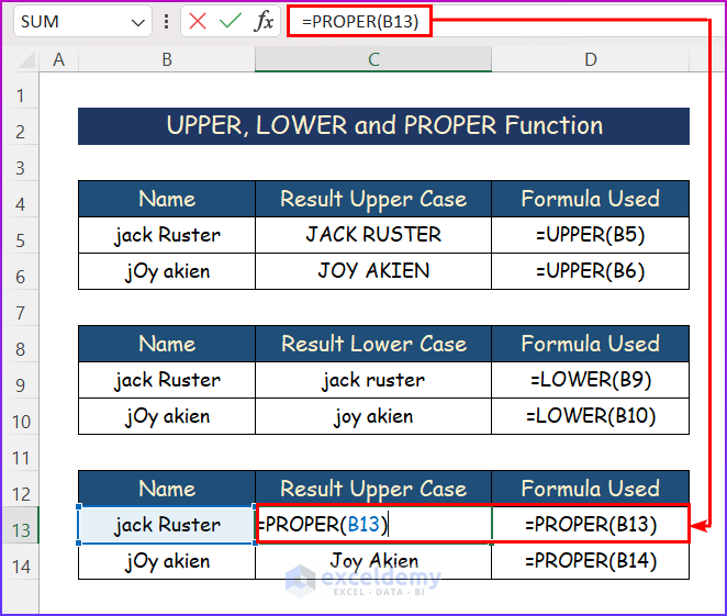
- Use the AutoFill tool to apply the same formula to the remaining cells.
Function Type 2 – CHAR Substring Function: Syntax and Arguments
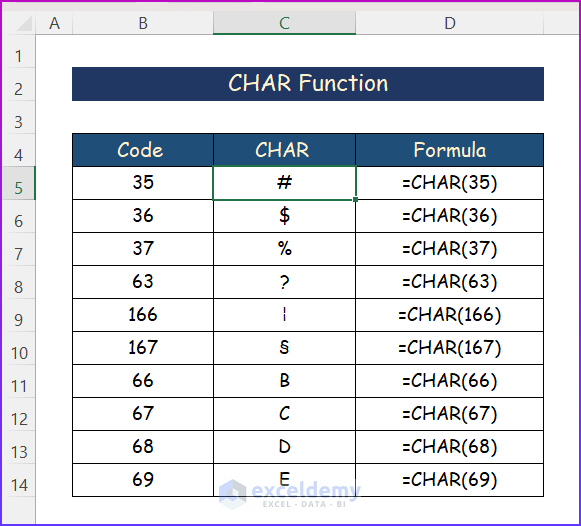
The CHAR function can convert a number (from 1 to 255) into ASCII characters. For example, CHAR(65) returns A, and CHAR(66) returns B. The CHAR function is useful when you want to enter characters that are difficult to insert directly.
Syntax:
=CHAR(number)
Arguments:
The syntax has only one argument. It is a required argument or parameter.
| Argument | Required/Optional | Explanation |
|---|---|---|
| number | Required | A number between 1 to 255 assigned to a specific character. |
Example of CHAR Function
Steps:
- Enter the code number.
- Select a cell and insert the following formula.
=CHAR(B5)
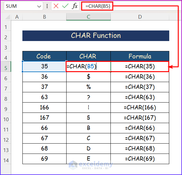
- Press Enter to get the desired character.
Read More: Excel Formula to Replace Text with Number
Function Type 3 – REPLACE Function: Syntax and Arguments
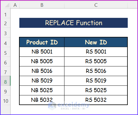
The REPLACE function is used to replace a part of a text string with a different text string. The function returns with the new text string within which new and replaced text or word is present.
Syntax:
=REPLACE(old_text, start_num, num_chars, new_text)
Arguments:
The syntax has four arguments. All are required arguments or parameters.
| Argument | Required/Optional | Explanation |
|---|---|---|
| old_text | Required | The text within which a part has to be replaced. |
| start_num | Required | The starting number of the character of the part that has to be replaced. |
| num_chars | Required | The number of characters that have to be replaced with a new text. |
| new_text | Required | The text that has to be added by replacing the old one in the text string. |
Example of REPLACE Function
Let’s replace the initial part of the product ID in the sample dataset.
Steps:
- Select a cell.
- Enter the following formula.
=REPLACE(B5,1,2,”RS”)
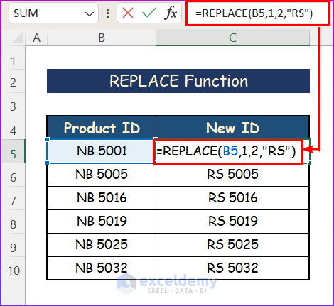
- Press Enter and the previous ID will be replaced by the new ID.
Read More: Excel VBA: How to Replace Text in String
Function Type 4 – TRIM Substring Function: Syntax and Arguments
The TRIM function can be used to remove all spaces from a text string except for single spaces between words. The TRIM function can remove leading and trailing spaces. It can also replace multiple consecutive spaces with a single space.
Syntax:
=TRIM(text)
Arguments:
The syntax has only one argument. It is a required argument or parameter.
| Argument | Required/Optional | Explanation |
|---|---|---|
| text | Required | It is the main string of text. |
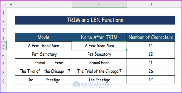
Example of TRIM Function
Steps:
- Select the cell where you want to apply the function.
- Enter the following formula.
=TRIM(B5)
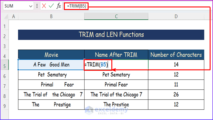
- Extra spaces will be removed.
Read More: How to Replace Text between Two Characters in Excel
Function Type 5 – LEN Function: Syntax and Arguments
The LEN function can be used to return the number of characters in a text string. This function works with numbers, but number formatting is not included.
Syntax:
=LEN(text)
Arguments:
The syntax has only one argument. It is a required argument or parameter.
| Argument | Required/Optional | Explanation |
|---|---|---|
| text | Required | It is the main string of text for which to calculate length. |
Example of LEN Function
Steps:
- Click on the cell named ‘Name After TRIM’.
- Enter the following formula in another cell.
=LEN(B5)
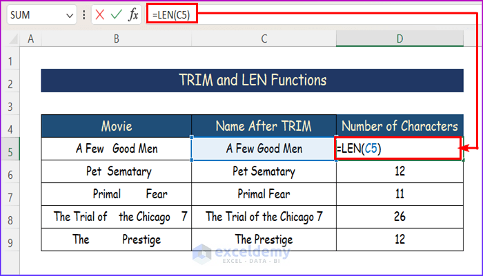
- Press Enter.
Read More: How to Split Text by Number of Characters in Excel
Function Type 6 – LEFT, RIGHT, and MID Functions: Syntax and Arguments
Functions such as LEFT, RIGHT, and MID can help you extract a word or text from another text string. The three substring functions in Excel will provide three different parts of a particular string.
6.1 LEFT Function
The LEFT function is categorized under the TEXT function in Excel. This function returns a specified number of characters from the start of the provided text string. The LEFT function returns the first num_chars characters in the text string.
Syntax:
=LEFT(text, [num_chars])
Arguments:
The syntax has also two arguments. Both are required arguments or parameters.
| Argument | Required/Optional | Explanation |
|---|---|---|
| text | Required | text is the main string where you want to apply the function. |
| num_chars | Required | num_chars is the number of characters that will be extracted during the operation. |
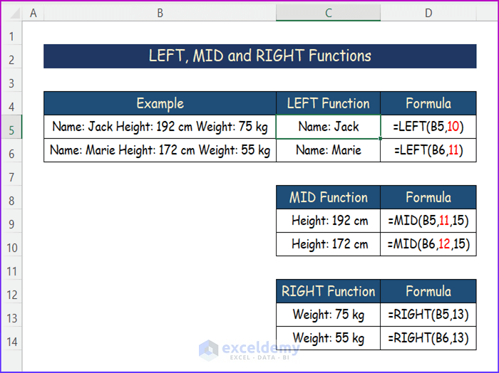
Example of LEFT Function
Steps:
- Click on a cell.
- Enter the following formula.
=LEFT(B5,10)
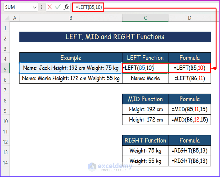
- Press Enter to get the left part of the sample data as shown in the image below.
Read More: How to Switch First and Last Name in Excel with Comma
6.2 RIGHT Function
The RIGHT function returns the last num_chars characters in the text string. It will extract digits from numbers as well as text.
Syntax:
=RIGHT(text, [num_chars])
Arguments:
The syntax has two arguments. Both are required arguments or parameters.
| Argument | Required/Optional | Explanation |
|---|---|---|
| text | Required | text is the main string where you want to apply the function. |
| num_chars | Required | num_chars is the number of characters that will be extracted during the operation. |
Example of RIGHT Function
Steps:
- Select a cell and enter the formula below.
=RIGHT(B5,13)
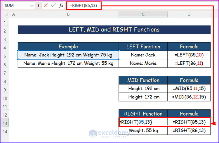
- The desired part of the data will be extracted.
Read More: How to Split String by Length in Excel
6.3 MID Function
The MID function returns a string containing a specified number of characters from the start position of a string. It is used to separate specific characters within a string.
Syntax:
=MID(text,start_num,num_chars)
Arguments:
The syntax has three arguments. All are required arguments or parameters.
| Argument | Required/Optional | Explanation |
|---|---|---|
| text | Required | The string from which characters will be extracted. It can be any text value, number, or array. |
| start_num | Required | The starting position from which characters will be extracted. It can be a single number or an array of numbers. |
| num_chars | Required | The total number of characters that will be extracted. It can be a single number or an array of numbers. |
Example of MID Function
Steps:
- Click on a cell.
- Enter the following formula into the cell.
=MID(B5,11,15)
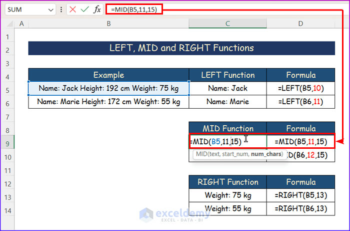
- Press Enter.
Read More: Excel VBA: Replace Character in String by Position
Function Type 7 – FIND/SEARCH Functions: Syntax and Arguments
7.1 FIND Function
In Microsoft Excel, the FIND function is generally used to extract the position of a defined text in a cell containing a text string. It returns the starting position of a case-sensitive text string within another text string.
Syntax:
=FIND(find_text, within_text, [start_num])
Arguments:
The syntax has three arguments. Two are required arguments or parameters and one is an optional argument.
| Argument | Required/Optional | Explanation |
|---|---|---|
| find_text | Required | A text or a part of a text to be searched for in a cell containing another text string. |
| within_text | Required | The cell containing the text is where the defined character or part of the text will be searched for. |
| [start_num] | Optional | Defined position in the text string from where the character count will be initiated. |
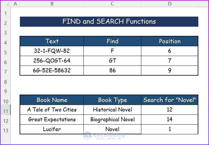
Example of FIND Function
Steps:
- Click on the cell named ‘Position’.
- Enter the following formula into the cell.
=FIND(C5,B5)
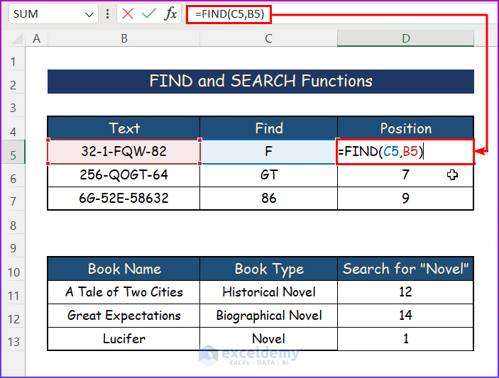
- It will return the position of the desired item from the sample data.
Read More: Excel VBA: How to Find and Replace Text in Word Document
7.2 SEARCH Function
In Microsoft Excel, the SEARCH function returns the number of characters at which a specific character or text string is first found, counting from left to right. It works for both array and non-array Formulas. The SEARCH function is not case-sensitive.
Syntax:
=SEARCH(find_text, within_text, [start_num])
Arguments:
The syntax has three arguments. Two are required arguments or parameters and one is an optional argument.
| Argument | Required/Optional | Explanation |
|---|---|---|
| find_text | Required | The text that is searched for. Can be a single text or an array of texts. |
| within_text | Required | The text value within which the find_text argument is searched for. Can be a single text value or an array of text values. |
| [start_num] | Optional | The position of the within_text argument from which it starts searching. It can be a single number or an array of numbers. Default is 1. |
Example of SEARCH Function
Steps:
- Click on a cell and enter the following formula in order to search for a particular item.
=SEARCH(“Novel”,C11,1)
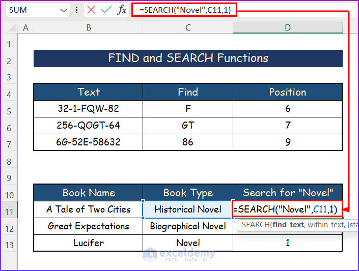
- Press Enter and it will return the position of the search keyword.
Read More: How to Replace Text after Specific Character in Excel
4 Examples to Extract Substring Before/After Specific Text or Character
We have combined multiple substring functions into a single dataset in Excel. We have divided it into three parts.
Example 1 – Combining UPPER, LEFT, and SEARCH Substring Functions
Steps:
- Select a cell other than the data set.
- Enter the formula in the formula bar.
=UPPER(LEFT(B5,SEARCH("-",B5,1)-1))
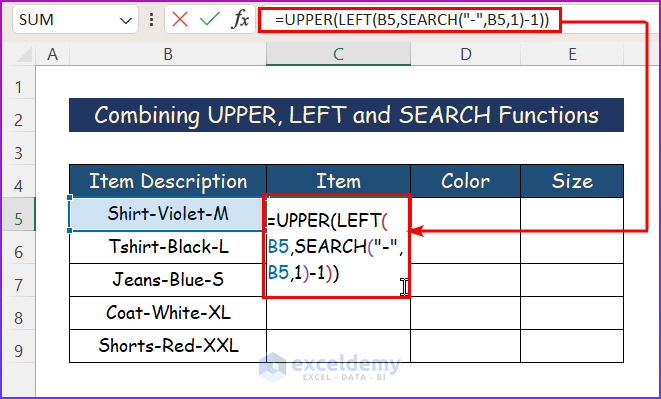
Formula Breakdown
- =UPPER(LEFT(B5,SEARCH(“-“,B5,1)-1))
- The UPPER function changes all lowercase letters to uppercase.
- The LEFT function provides the left part of the string.
- The SEARCH function will return the number of characters at which a specific character or text string is first found, reading from left to right. It will count characters up to “–”.
- We selected column B5.
- The formula will extract data and provide the output accordingly.
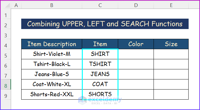
- Press Enter to get the left side of the data with all uppercase letters.
- Use the AutoFill tool for the remaining cells.
Read More: How to Replace Text in Selected Cells in Excel
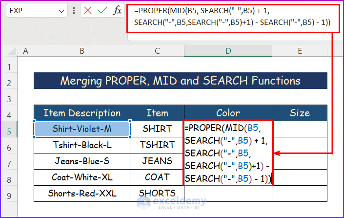
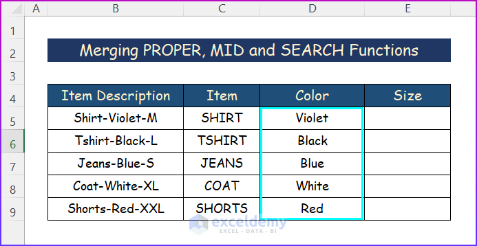
Example 2 – Merging PROPER, MID, and SEARCH Functions
Steps:
- Click on a cell.
- Enter the following formula.
=PROPER(MID(B5, SEARCH("-",B5) + 1, SEARCH("-",B5,SEARCH("-",B5)+1) - SEARCH("-",B5) - 1))
Formula Breakdown
- =PROPER(MID(B5, SEARCH(“-“,B5) + 1, SEARCH(“-“,B5,SEARCH(“-“,B5)+1) – SEARCH(“-“,B5) – 1))
- The PROPER function changes all letters to the proper case.
- The MID function provides the data from the middle part of the string.
- The SEARCH function will return the number of characters at which a specific character or text string is first found, reading from left to right. It will count characters up to “–”.
- We selected column B5.
- The formula will extract the middle part of the data and provide the output accordingly.
- Press Enter to get your final result.
Read More: How to Extract Text after Second Comma in Excel
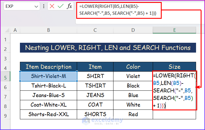
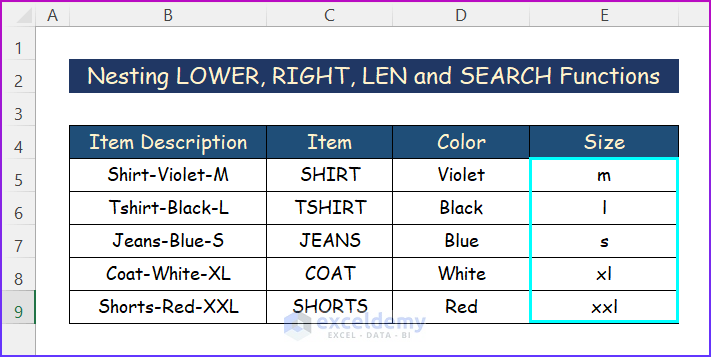
Example 3 – Nesting LOWER, RIGHT, LEN, and SEARCH Substring Functions
Steps:
- Click on cell and enter the following formula.
=LOWER(RIGHT(B5,LEN(B5)-SEARCH("-",B5, SEARCH("-",B5) + 1)))
Formula Breakdown
- =LOWER(RIGHT(B5,LEN(B5)-SEARCH(“-“,B5, SEARCH(“-“,B5) + 1)))
- The LOWER function changes all letters to the lowercase in a string.
- The RIGHT function provides the data from the extreme right part of the string.
- The LEN function returns the number of characters in a text string.
- The SEARCH function will return the number of characters at which a specific character or text string is first found, reading from left to right.
- It will count characters up to “–”. We selected column B5.
- The formula will extract the right part of the data and provide the output in lowercase.
- Press Enter.
- You will get the desired output result as below.
Read More: How to Extract Text after a Specific Text in Excel
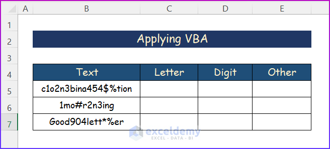
Example 4 – Applying VBA to Extract Substring
When letters and digits are placed together in a way that you cannot find a rule to split them easily, you can use the VBA code to complete the task. It can be applied to multiple substring functions in Excel.
Steps:
- Open the worksheet where you want the text to be split.
- Press Alt+F11 to open the Microsoft Visual Basic Applications.
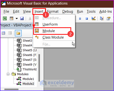
- Go to Insert.
- Click on Module from the menu to create a module.
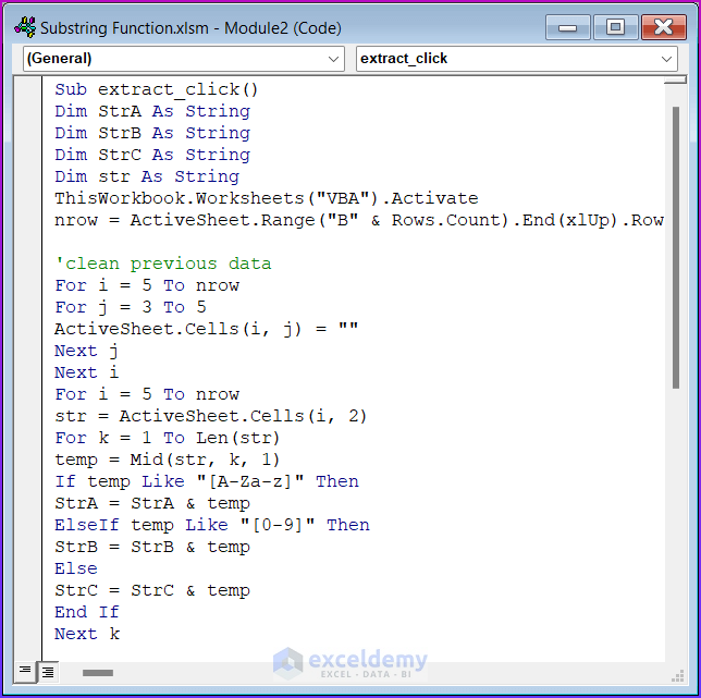
- A new window will open. Enter the following VBA macro in the Module.
Sub extract_click() Dim StrA As String Dim StrB As String Dim StrC As String Dim str As String ThisWorkbook.Worksheets("VBA").Activate nrow = ActiveSheet.Range("B" & Rows.Count).End(xlUp).Row 'Exceldemy Publications For i = 5 To nrow For j = 3 To 5 ActiveSheet.Cells(i, j) = "" Next j Next i For i = 5 To nrow str = ActiveSheet.Cells(i, 2) For k = 1 To Len(str) temp = Mid(str, k, 1) If temp Like "[A-Za-z]" Then StrA = StrA & temp ElseIf temp Like "[0-9]" Then StrB = StrB & temp Else StrC = StrC & temp End If Next k ActiveSheet.Cells(i, 3) = StrA ActiveSheet.Cells(i, 4) = StrB ActiveSheet.Cells(i, 5) = StrC StrA = "" StrB = "" StrC = "" Next i EndSub
VBA Code Breakdown
- We create a new procedure Sub in the worksheet using the below statement.
Sub extract_click()
- We declare variables as
Dim StrA As String
Dim StrB As String
Dim StrC As String
Dim str As String- We activate the VBA sheet and select the range for nrow.
ThisWorkbook.Worksheets("VBA").Activate
nrow = ActiveSheet.Range("B" & Rows.Count).End(xlUp).Row- We applied the For loop to i and j.
For i = 5 To nrow
For j = 3 To 5
ActiveSheet.Cells(i, j) = ""
Next j
Next i- We applied two For loops and declared 4 strings- str, StrA, StrB and StrC.
For i = 5 To nrow
str = ActiveSheet.Cells(i, 2)
For k = 1 To Len(str)
temp = Mid(str, k, 1)
If temp Like "[A-Za-z]" Then
StrA = StrA & temp
ElseIf temp Like "[0-9]" Then
StrB = StrB & temp
Else
StrC = StrC & temp- We started an END If function and activated the cells according to the strings.
End If
Next k
ActiveSheet.Cells(i, 3) = StrA
ActiveSheet.Cells(i, 4) = StrB
ActiveSheet.Cells(i, 5) = StrC
StrA = ""
StrB = ""
StrC = ""
Next i- We end the Sub of the VBA macro as
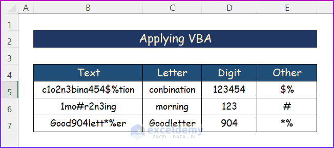
End Sub- Press F5 to run the VBA.
- You will get the split data in the desired columns.
Read More: Find and Replace a Text in a Range with Excel VBA
Download Practice Workbook
Related Articles
- How to Extract Certain Text from a Cell in Excel VBA
- Excel VBA to Replace Blank Cells with Text (3 Examples)
- Excel VBA to Find and Replace Text in a Column
- Split Text in Excel into Multiple Rows
- How to Separate Text in Excel


Please check the .pdf link.
It leads to “Extract Data from a Webpage to Excel” instead to the post above.
Regards Roger
Roger, thanks a lot. I did not notify the issue. It’s a crucial problem. I am working on it.