This tutorial will demonstrate 5 simple methods to replace text with a blank cell in Excel. When working with a dataset, we may need to eliminate specific cell values. Sometimes we have to replace text in certain cells with blank cells. To make you understand better we will illustrate the methods with a unique dataset.
How to Replace Text with Blank Cell in Excel: 5 Simple Methods
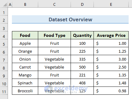
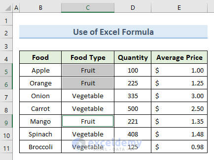
This article will discuss the 5 possible ways to replace text with a blank cell in Excel. We will use the following dataset to illustrate the methods of this article. The dataset includes two columns Food and Food Type. We also get the Price and Average Price of different foods from the dataset. In the given dataset, we will replace the cell value Fruit with blank cells.
1. Apply Ribbon to Replace Text with Blank Cell
In the first method, we will use the Excel ribbon to replace text with a blank cell. Using the ‘Find & Select’ option in the ribbon we can replace any text from our dataset. To replace a text from a dataset with a blank cell follow the below steps.
STEPS:
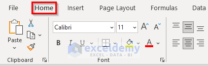
- To begin with, go to the Home tab.
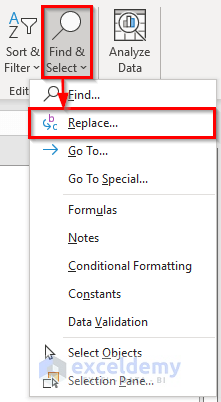
- In addition, select the option ‘Find & Select’ from the ribbon.
- Furthermore, from the dropdown menu select the option Replace.
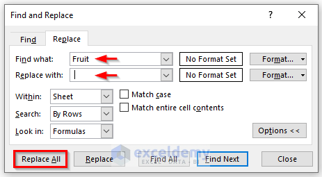
- The above action opens a new dialogue box named ‘Find and Replace’.
- Next, type the value Fruit in the ‘Find what’ text field.
- Then, type a space in the ‘Replace with’ text field.
- After that, click on the Replace All button.
- Lastly, we can see our desired result in the following image.
![]()
Read More: How to Replace Text in Selected Cells in Excel
2. Replace Text with Blank Cell Using Excel Formula
Another simple method to replace text with a blank cell is to use the Excel formula. In this method, we will use a simple formula that will replace specific text with blank cells. Let’s see the steps to do it.
STEPS:
- First, select all the cells that contain the text Fruit.
- Next, press F2 or place the cursor in the formula bar.
- Then, type the following formula:
=""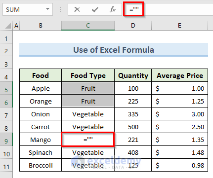
- Now, press Ctrl + Enter.
- Finally, we can see that the above formula replaces the text Fruit with blank cells.
![]()
Read More: Excel Formula to Replace Text with Number
3. Apply REPLACE Function to Replace Text with Blank Cell in Excel
In this method, we will use the REPLACE function to fill in the specific text with a blank cell. The REPLACE function in Excel replaces characters in a text string indicated by location with characters from another text string. In our dataset, we will create a duplicate of the Food Type column. In the new column, we will replace the text Fruit with blank cells. Let’s see the steps to use this function.
STEPS:
- Firstly, select cell F5.
- Secondly, type the following formula in that cell:
=REPLACE(C5,1,5,"")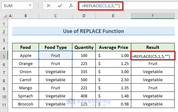
- Press Enter.
- So, the above formula replaces the text in cell F5 with a blank cell.
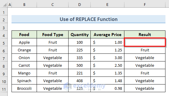
- After that, use the formulas in cells F6 and F9 that we can see in the image below.
- In the end, after using these formulas we get our desired result like the following image.
Read More: How to Replace Text between Two Characters in Excel
4. Replace Text with Blank Cells Using SUBSTITUTE Function
We can also use the SUBSTITUTE function to replace text with blank cells. The SUBSTITUTE function in Excel matches the text in a string and replaces it. Let’s see the steps to this method.
STEPS:
- In the first place, select cell F5.
- Next, type the following formula in that cell:
=SUBSTITUTE(C5,"Fruit","")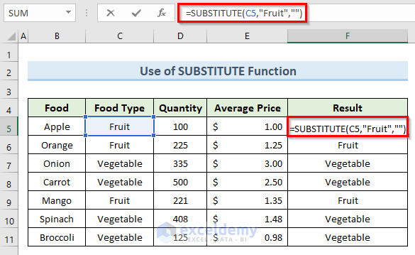
- Press, Enter.
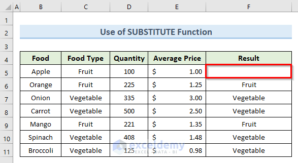
- So, the above formula returns a blank value in cell F5.
- Afterward, type the formulas like the following image in cells F6 and F9.
- Finally, the above formulas replace the text value Fruit with blank cells like the following image.
Read More: How to Replace Text after Specific Character in Excel
5. Utilize ‘Go To Special’ Option to Substitute Text with Blank Cell
In the last method, we will replace text with a blank cell using the ‘Go To Special’ option. This method is only applicable for the same type of data. To illustrate this method we have inserted a new column with our dataset. The new column represents the total price of products. Here, the total price is the product of the value of quantity and average price. So, all the values in the column Total Price consist of formulas. We will use the ‘Go To Special’ option only to replace the text that we get using the formula.

Let’s see the steps to perform this method.
STEPS:
- To begin with, go to the Formulas tab. Select the option ‘Show Formulas’.

- We can see the used formulas in our dataset from cells (E5:E11). These are the values that we will replace with blank cells.

- In addition, go to the Formulas tab again. Deselect the option ‘Show Formulas’. So, we will get our dataset in the previous condition.

- Next, go to the Home tab.

- Then, select the option ‘Find & Select’ from the ribbon.
- Afterward, from the dropdown menu select the option ‘Go To Special’.
![]()
- A new dialogue box named ‘Go To Special’ will appear. We can also open that dialogue box by firstly pressing Ctrl + G. Then, click on the Special.
- Furthermore, check the option Formulas and click on OK.
![]()
- The above action selects all the cells that contain a formula.
- Moreover, press F2 or place the cursor in the formula bar.
- After that, type the following formula:
=""![]()
- Press, Ctrl + Enter.
- Lastly, we get the result like the following image.
![]()
Read More: How to Replace Text with Carriage Return in Excel
Download Practice Workbook
You can download the practice workbook from here.
Conclusion
In conclusion, this tutorial shows 5 simple ways to replace text with blank cells. To put your skills to the test, use the sample worksheet provided in this article. Please leave a comment in the box below if you have any questions. Our team will make every effort to respond to your message as quickly as possible. In the future, keep an eye out for more innovative Microsoft Excel solutions.
<< Go Back to Excel REPLACE Function | Excel Functions | Learn Excel
Get FREE Advanced Excel Exercises with Solutions!
