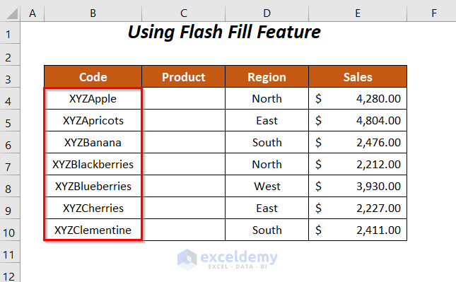
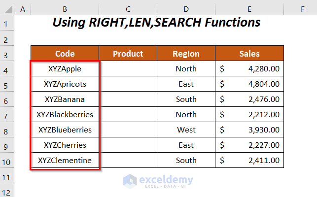
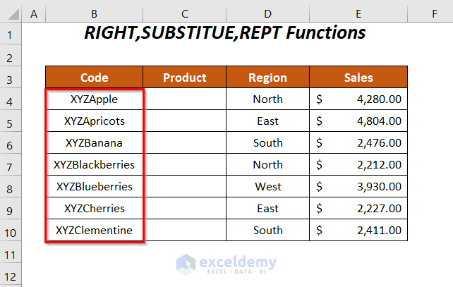
Method 1 – Using Flash Fill Feature to Extract Text after a Specific Text
Steps:
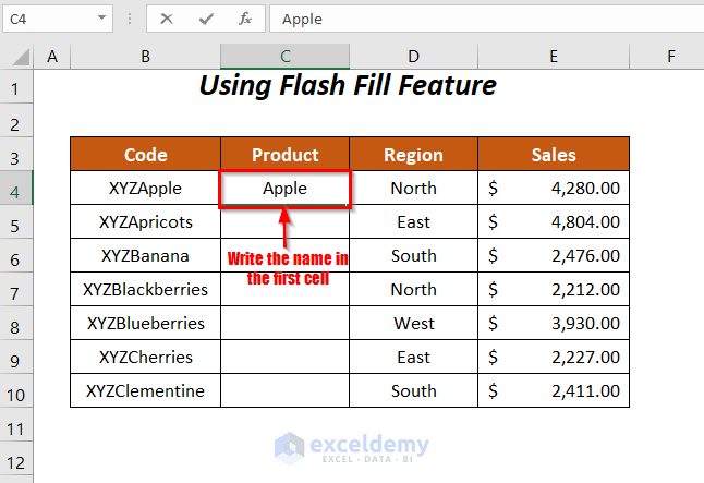
- Enter the product name, Apple, from the code in cell C4.
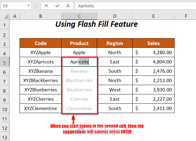
- Enter the second product’s name Apricots in cell C5. Flash Fill feature will show suggestions.
- Press ENTER.
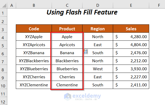
- The result will show the name of the products extracted from the codes after the text XYZ.
Read More: How to Extract Text Before Character in Excel
Method 2 – Using the Combination of the RIGHT, LEN, and SEARCH Functions
Steps:
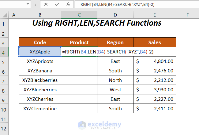
- Add the following formula in cell C4.
=RIGHT(B4,LEN(B4)-SEARCH("XYZ",B4)-2)B4 is the product code.
Formula Breakdown
- LEN(B4) becomes
LEN(“XYZApple”) → gives the total number of characters in this text string.
Output → 8
- SEARCH(“XYZ”,B4) becomes
SEARCH(“XYZ”, “XYZApple”) → searches for the text XYZ in XYZApple and gives the position of the first character X in the string.
Output → 1
- LEN(B4)-SEARCH(“XYZ”,B4) becomes
8-1 → 7
- LEN(B4)-SEARCH(“XYZ”, B4)-2 becomes
7-2 → subtracts 2 from the number of texts 7 because of omitting the remainder YZ of XYZ also.
Output → 5
- RIGHT(B4,LEN(B4)-SEARCH(“XYZ”,B4)-2) becomes
RIGHT(“XYZApple”,5) → extracts 5 characters from the right side.
Output → Apple
- Press ENTER and drag down the Fill Handle tool.
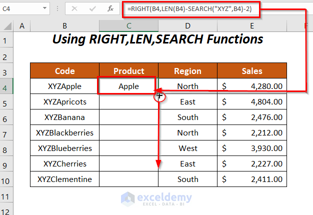
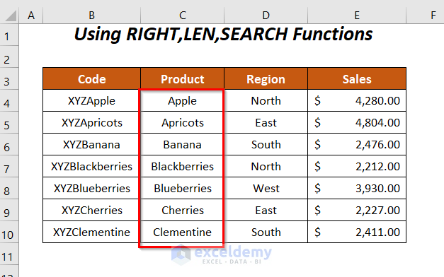
- The result will show all the product names in the Product column.
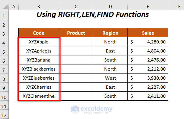
Method 3 – Extract Text after a Specific Text Using the RIGHT, LEN, and FIND Functions
Steps:
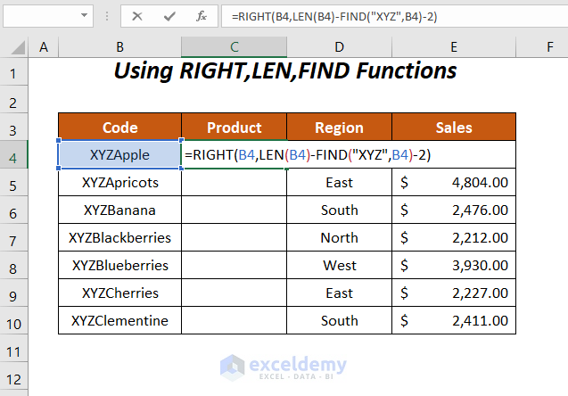
- Add the following formula in cell C4.
=RIGHT(B4,LEN(B4)-FIND("XYZ",B4)-2)B4 is the product code.
Formula Breakdown
- LEN(B4) becomes
LEN(“XYZApple”) → gives the total number of characters in this text string.
Output → 8
- FIND(“XYZ”,B4) becomes
FIND(“XYZ”, “XYZApple”) → searches for the text XYZ in XYZApple and gives the position of the first character X in the string.
Output → 1
- LEN(B4)-FIND(“XYZ”,B4) becomes
8-1 → 7
- LEN(B4)-FIND(“XYZ”, B4)-2 becomes
7-2 → subtracts 2 from the number of texts 7 because of omitting the remainder YZ of XYZ also.
Output → 5
- RIGHT(B4,LEN(B4)-FIND(“XYZ”,B4)-2) becomes
RIGHT(“XYZApple”,5) → extracts 5 characters from the right side.
Output → Apple
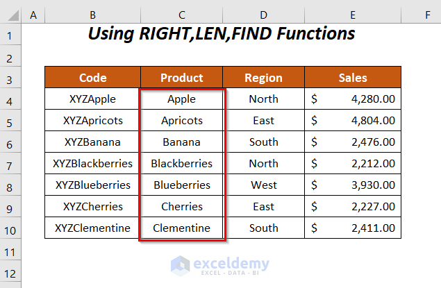
- Press ENTER and drag down the Fill Handle tool.
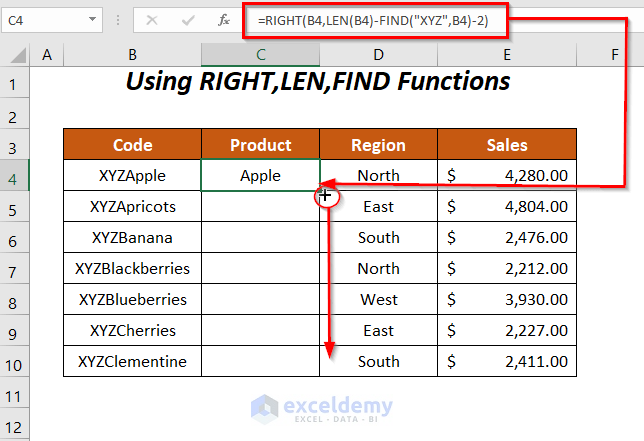
- It will output the product names in the Product column extracting them after the text XYZ from the codes.
Read More: How to Extract Text After First Space in Excel
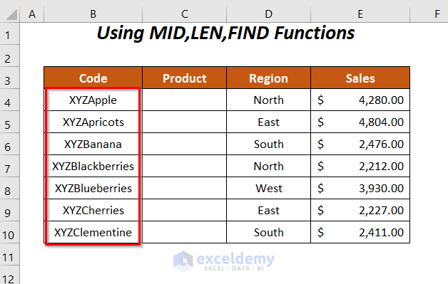
Method 4 – Using the Combination of MID, LEN, FIND Functions to Extract Text after a Specific Text
Steps:
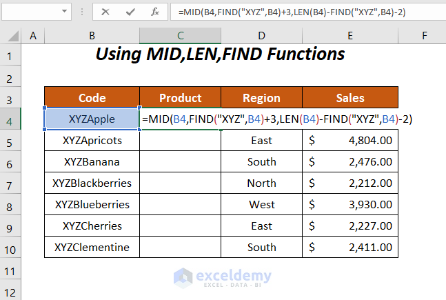
- Add the following formula in cell C4.
=MID(B4,FIND("XYZ",B4)+3,LEN(B4)-FIND("XYZ",B4)-2)B4 is the product code.
Formula Breakdown
- FIND(“XYZ”,B4) becomes
FIND(“XYZ”, “XYZApple”) → searches for the text XYZ in XYZApple and gives the position of the first character X in the string.
Output → 1
- FIND(“XYZ”,B4)+3 becomes
1+3 → 3 is added to get the starting position of the text that we want to draw out after XYZ.
Output → 4
- LEN(B4) becomes
LEN(“XYZApple”) → gives the total number of characters in this text string.
Output → 8
- LEN(B4)-FIND(“XYZ”,B4) becomes
8-1 → 7
- LEN(B4)-FIND(“XYZ”, B4)-2 becomes
7-2 → subtracts 2 from the number of texts 7 because of omitting the remainder YZ of XYZ also.
Output → 5
- MID(B4,FIND(“XYZ”,B4)+3,LEN(B4)-FIND(“XYZ”,B4)-2) becomes
MID(“XYZApple”,4,5) → extracts the part starting from position 4 and the total length of the characters would be 5.
Output → Apple
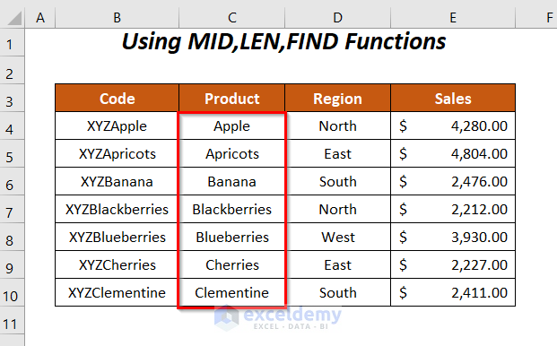
- Press ENTER and drag down the Fill Handle tool.
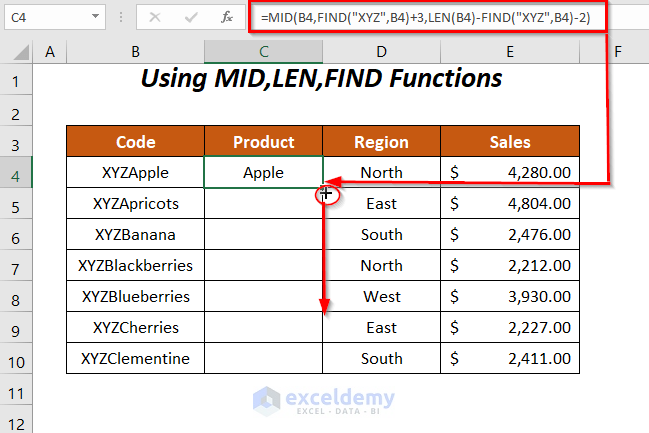
- The result will show the products’ names in the Product column.
Method 5 – Extract Text after a Specific Text Using the SUBSTITUTE, LEFT, and FIND Functions
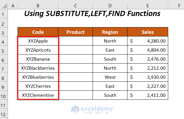
Steps:
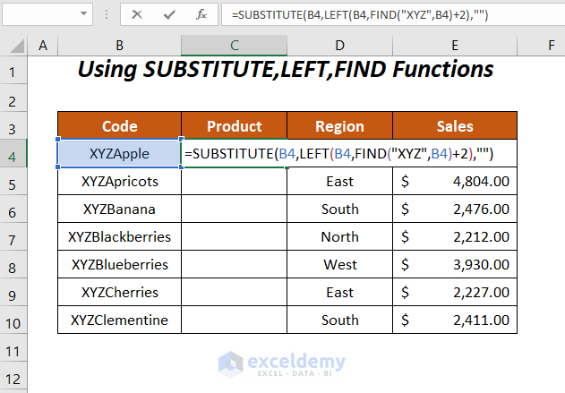
- Add the following formula in cell C4.
=SUBSTITUTE(B4,LEFT(B4,FIND("XYZ",B4)+2),"")B4 is the product code.
Formula Breakdown
- FIND(“XYZ”,B4) becomes
FIND(“XYZ”, “XYZApple”) → searches for the text XYZ in XYZApple and gives the position of the first character X in the string.
Output → 1
- FIND(“XYZ”,B4)+2 becomes
1+2 → 2 is added to get the total number of characters in text XYZ.
Output → 3
- LEFT(B4,FIND(“XYZ”,B4)+2) becomes
LEFT(“XYZApple”,3) → draws out the first 3 characters from the left of this string.
Output → “XYZ”
- SUBSTITUTE(B4,LEFT(B4,FIND(“XYZ”,B4)+2),””) becomes
SUBSTITUTE(“XYZApple”, “XYZ”,””) → supersedes the part XYZ with a blank in the text XYZApple.
Output → Apple
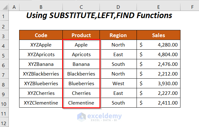
- Press ENTER and drag down the Fill Handle tool.
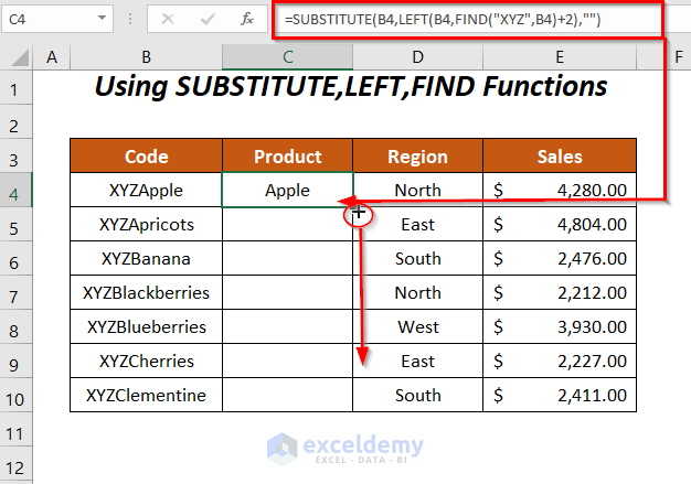
- The result will show the name of the products.
Method 6 – Using the SUBSTITUTE, RIGHT, and FIND Functions
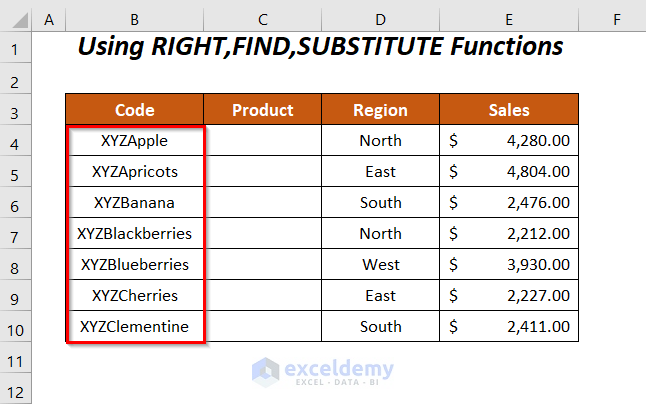
Steps:
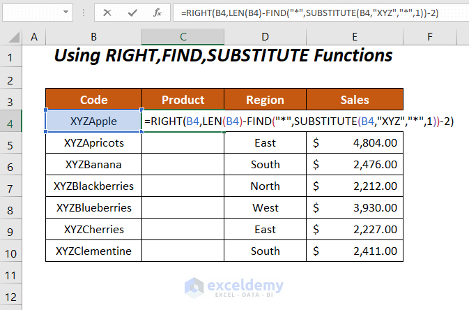
- Add the following formula in cell C4.
=RIGHT(B4,LEN(B4)-FIND("*",SUBSTITUTE(B4,"XYZ","*",1))-2)B4 is the product code.
Formula Breakdown
- LEN(B4) becomes
LEN(“XYZApple”) → gives the total number of characters in this text string.
Output → 8
- SUBSTITUTE(B4,”XYZ”,”*”,1) becomes
SUBSTITUTE(“XYZApple”, “XYZ”,”*”,1) → replaces the string XYZ with the * symbol and 1 is for the first occurrence.
Output → *Apple
- FIND(“*”,SUBSTITUTE(B4,”XYZ”,”*”,1)) becomes
FIND(“*”,*Apple) → finds the position of the * symbol in the string
Output → 1
- LEN(B4)-FIND(“*”,SUBSTITUTE(B4,”XYZ”,”*”,1)) becomes
8-1 → 7
- FIND(“*”,SUBSTITUTE(B4,”XYZ”,”*”,1))-2 becomes
7-2 → subtracts 2 from the number of texts 7 because of omitting the remainder YZ of XYZ also.
Output → 5
- RIGHT(B4,LEN(B4)-FIND(“*”,SUBSTITUTE(B4,”XYZ”,”*”,1))-2) becomes
RIGHT(“XYZApple”,5) → extracts 5 characters from the right side.
Output → Apple
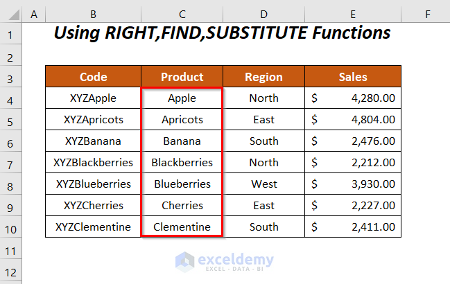
- Press ENTER and drag down the Fill Handle tool.
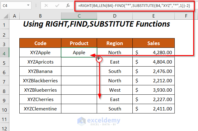
- The result will show the product names in the Product column.
Similar Readings
- How to Extract Text after Second Space in Excel
- How to Extract Text After Last Space in Excel
- How to Extract Text Between Two Commas in Excel
Method 7 – Using the REPLACE Function to Extract Text after a Specific Text
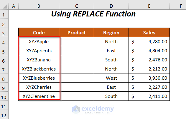
Steps:
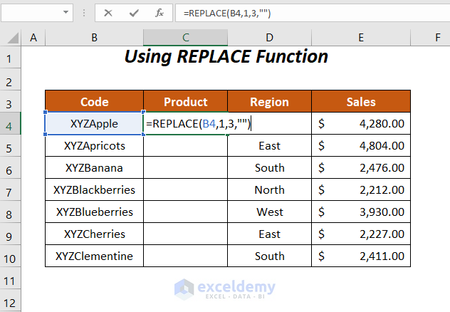
- Add the following formula in cell C4.
=REPLACE(B4,1,3,"")B4 is the product code. REPLACE will supersede the string which starts from position 1 and has a length of 3 with a blank.
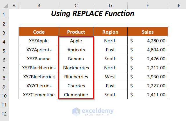
- Press ENTER and drag down the Fill Handle tool.
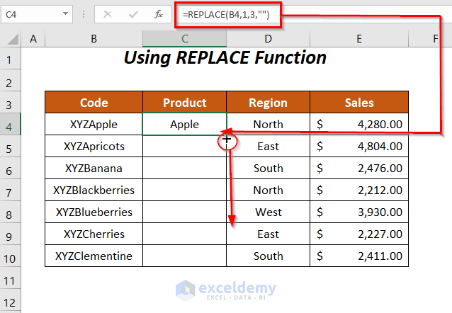
- The result will show the name of the products.
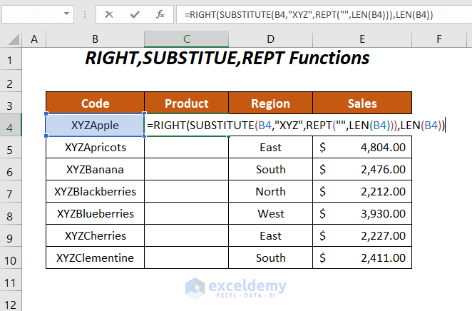
Method 8 – Use the RIGHT, SUBSTITUTE, and REPT Functions to Extract Text after a Specific Text
Steps:
- Add the following formula in cell C4.
=RIGHT(SUBSTITUTE(B4,"XYZ",REPT("",LEN(B4))),LEN(B4))B4 is the product code.
Formula Breakdown
- LEN(B4) becomes
LEN(“XYZApple”) → gives the total number of characters in this text string.
Output → 8
- REPT(“”,LEN(B4))) becomes
REPT(“”,8) → returns blank
Output → “”
- SUBSTITUTE(B4,”XYZ”,REPT(“”,LEN(B4))) becomes
SUBSTITUTE(“XYZApple”, “XYZ”,””) → replaces the part XYZ with a blank in the text XYZApple.
Output → “Apple”
- RIGHT(SUBSTITUTE(B4,”XYZ”,REPT(“”,LEN(B4))),LEN(B4)) becomes
RIGHT(“Apple”,8) → returns characters up to 8 lengths from the right as there is 5 character it will return 5 characters.
Output → Apple
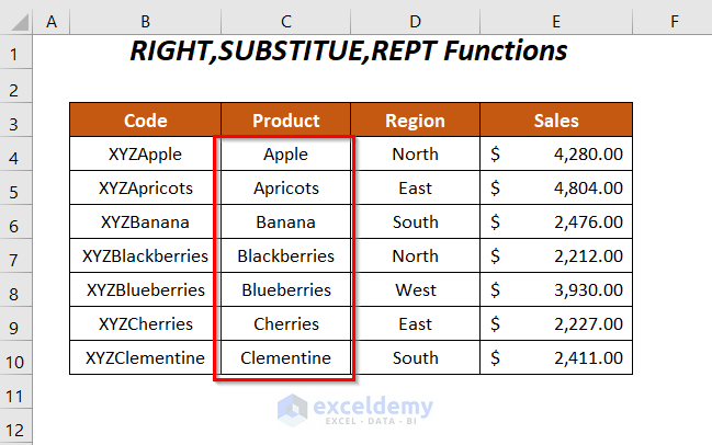
- Press ENTER and drag down the Fill Handle tool.
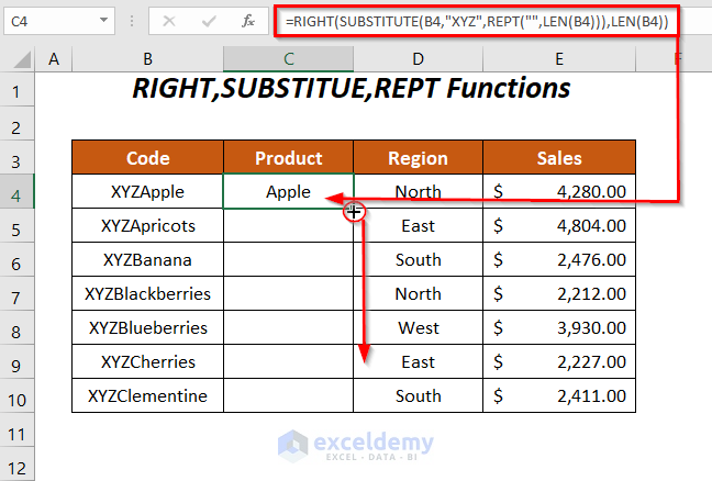
- The result will show the product names in the Product column.
Method 9 – Using the Text to Columns Option
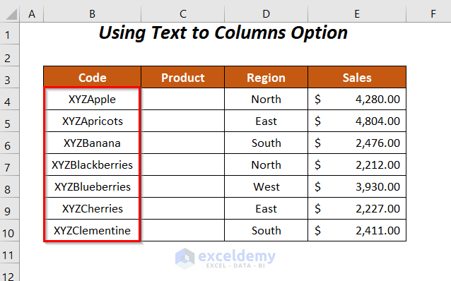
Steps:
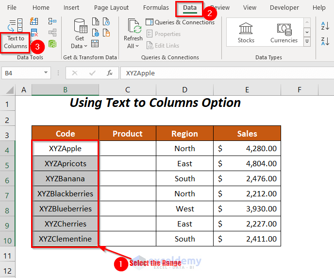
- Select the range and go to the Data Tab >> Data Tools Group >> Text to Columns Option.
- The Convert Text to Columns Wizard will appear.
- Click on the Fixed width option and press Next.
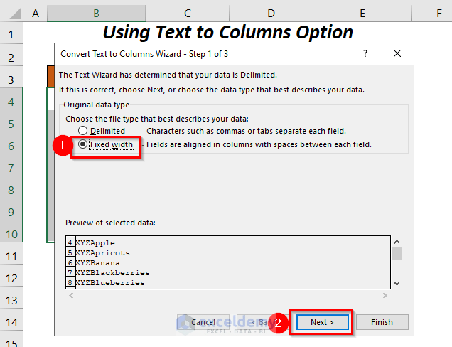
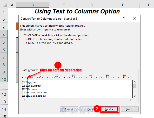
- You will be taken to Step-2 of the wizard.
- Click on the position where you want the separation (We want to have the division after XYZ so we have clicked next to it).
- Press Next.
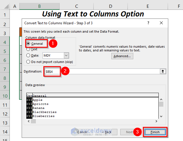
- Select and enter the following.
Column data format → General
Destination → $B$4 - Press Finish.
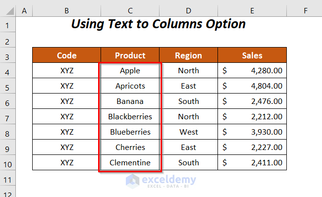
- The result will show the separated data and the names of the products will be in the Product column.
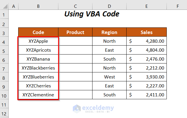
Method 10 – Using VBA Code to Extract Text after a Specific Text
Steps:
- Go to the Developer Tab >> Visual Basic Option.
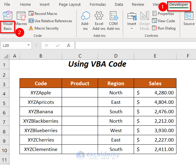
- The Visual Basic Editor will open up.
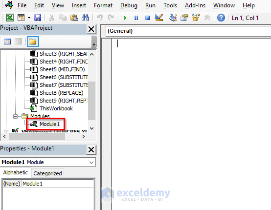
- Go to the Insert Tab >> Module Option.
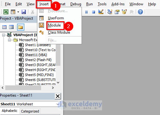
- A Module will be created.
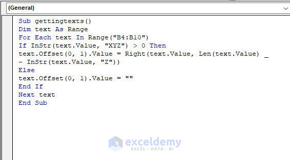
- Add the following code
Sub gettingtexts()
Dim text As Range
For Each text In Range("B4:B10")
If InStr(text.Value, "XYZ") > 0 Then
text.Offset(0, 1).Value = Right(text.Value, Len(text.Value) _
- InStr(text.Value, "Z"))
Else
text.Offset(0, 1).Value = ""
End If
Next text
End Sub
We have declared text as Range, and it will store each value of the cells for the range B4:B10 within the FOR loop. IF statement will check whether the values contain a specific portion XYZ with the help of the InStr function which looks for a partial match.
For matching the criteria we will extract the portion after XYZ from the texts in the adjacent cells.
- Press F5.

Download Workbook
Related Readings
- How to Extract Text after Second Comma in Excel
- How to Extract Text between Two Spaces in Excel
- How to Extract Text Between Two Characters in Excel
- How to Extract Certain Text from a Cell in Excel VBA
- How to Extract Text After a Character in Excel
<< Go Back to Extract Text in Excel | String Manipulation | Learn Excel
Get FREE Advanced Excel Exercises with Solutions!
