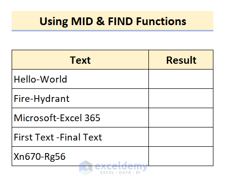
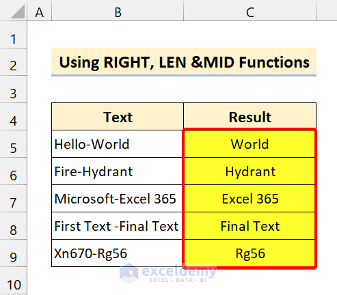
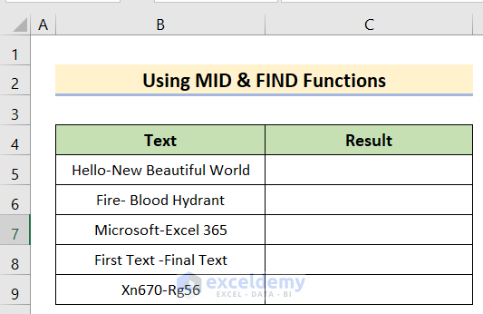
Method 1 – Using MID and FIND Functions to Extract Text After a Character
We’ll use the following dataset. We’ll extract the text after the hyphen (“-”).
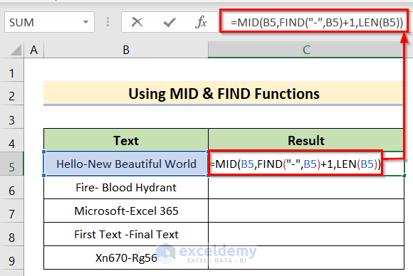
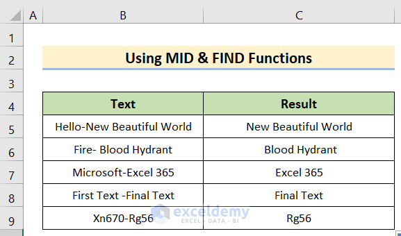
Steps
- Insert the following formula in Cell C5:
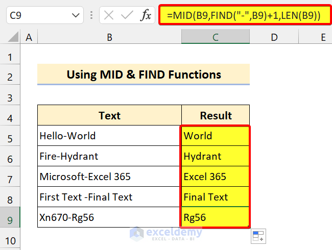
=MID(B5,FIND("-",B5)+1,LEN(B5))
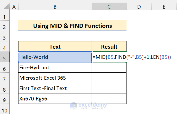
- Press Enter.
- Drag the Fill handle icon over the range of cells C5:C9.
Breakdown of the Formula
- LEN(B5) returns 11.
- FIND(“-“,B5) returns 6.
- MID(B5,FIND(“-“,B5)+1,LEN(B5)) = MID(B5,6+1,11) returns World.
Read More: How to Extract Text Before Character in Excel
Method 2 – Applying RIGHT, LEN, and FIND Functions to Extract Text After a Character
We’ll use the same dataset as in Method 1 and extract the text after the hyphen.
Steps
- Use the following formula in Cell C5:
=RIGHT(B5,LEN(B5)-FIND("-",B5))
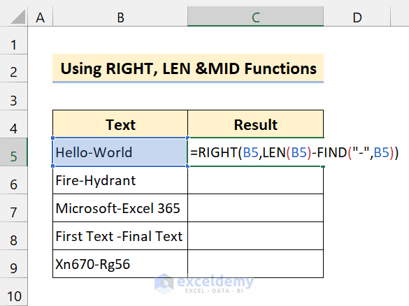
- Press Enter.
- Drag the Fill handle icon down to C9.
Breakdown of the Formula
- LEN(B5) returns 11.
- FIND(“-“,B5) returns 6.
- RIGHT(B5,LEN(B5)-FIND(“-“,B5)) =RIGHT(B5,11-6) returns World.
Read More: How to Extract Text after a Specific Text in Excel
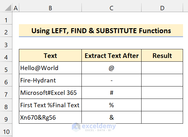
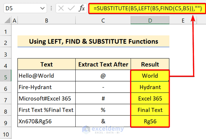
Method 3 – Using LEFT, FIND, and SUBSTITUTE Functions to Extract Text After a Character
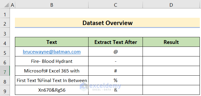
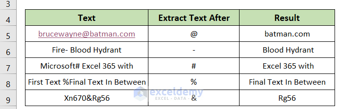
We are using the previous dataset, but we changed the lookup characters. We’ll extract the text from the cells after the character noted in the cell next to it.
Steps
- Use the following formula in Cell D5:
=SUBSTITUTE(B5,LEFT(B5,FIND(C5,B5)),"")
- Press Enter.
- Drag down the Fill handle icon to fill all the other cells in the column.
Breakdown of the Formula
- FIND(C5,B5) returns 6.
- LEFT(B5,6) returns Hello@.
- SUBSTITUTE(B5,LEFT(B5,FIND(C5,B5)),””) = SUBSTITUTE(B5,”Hello@”,””) returns World.
Read More: How to Extract Text After First Space in Excel
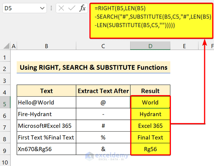
Method 4 – Combining RIGHT, SEARCH, and SUBSTITUTE Functions to Extract Specific Characters
Steps
- Use the following formula in Cell D5:
=RIGHT(B5,LEN(B5)-SEARCH("#",SUBSTITUTE(B5,C5,"#",LEN(B5)-LEN(SUBSTITUTE(B5,C5,"")))))
- Press Enter.
- Drag the Fill handle icon over the range of cells D6:D9.
Breakdown of the Formula
- LEN(B5) returns 11
- SUBSTITUTE(B5,C5,””) returns HelloWorld.
- SUBSTITUTE(B5,C5,”#”,11-LEN(“HelloWorld”)) returns Hello#World.
- SEARCH(“#”,”Hello#World”) returns 6.
- RIGHT(B5,LEN(B5)-SEARCH(“#”,SUBSTITUTE(B5,C5,”#”,LEN(B5)-LEN(SUBSTITUTE(B5,C5,””))))) = RIGHT(B5,11-6) returns World.
Read More: How to Extract Text after Second Space in Excel
Method 5 – Using RIGHT, SUBSTITUTE, and REPT Functions to Extract Text After a Character
Steps
- Use the following formula in Cell D5:
=TRIM(RIGHT(SUBSTITUTE(B5,C5,REPT(" ",LEN(B5))),LEN(B5)))
We used the TRIM function to remove extra leading spaces.
- Press Enter.
- Drag the Fill handle icon over the range of cells D6:D9.
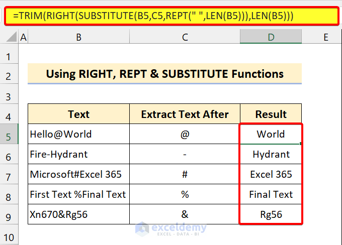
Breakdown of the Formula
- LEN(B5) returns 11
- REPT(” “,LEN(B5)) returns “ “ (Spaces).
- SUBSTITUTE(B5,C5,REPT(” “,LEN(B5))) returns “Hello World”.
- RIGHT(SUBSTITUTE(B5,C5,REPT(” “,LEN(B5))),LEN(B5)) returns “ World”.
- TRIM(RIGHT(SUBSTITUTE(B5,C5,REPT(” “,LEN(B5))),LEN(B5))) = TRIM(” World”) returns World.
Read More: How to Extract Text After Last Space in Excel
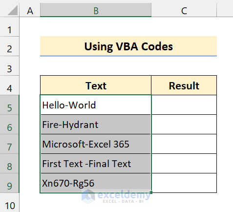
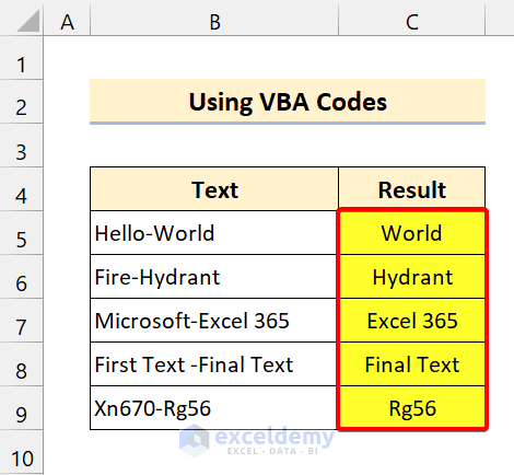
Method 6 – Inserting VBA Code to Extract Text After a Character in Excel
Steps
- Press Alt + F11 to open the VBA editor.
- Select Insert and choose Module.
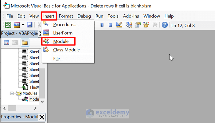
- Insert the following code in the code window.
Sub extract_text()

Dim rng As Range
Dim cell As Range
Set rng = Application.Selection
For Each cell In rng
 cell.Offset(0, 1).Value = Right(cell, Len(cell) - InStr(cell, "-"))
Next cell

End Sub- Save the file.
- Select the range of cells B5:B9.
- Press Alt + F8 to open the Macro dialog box.
- Select extract_text.
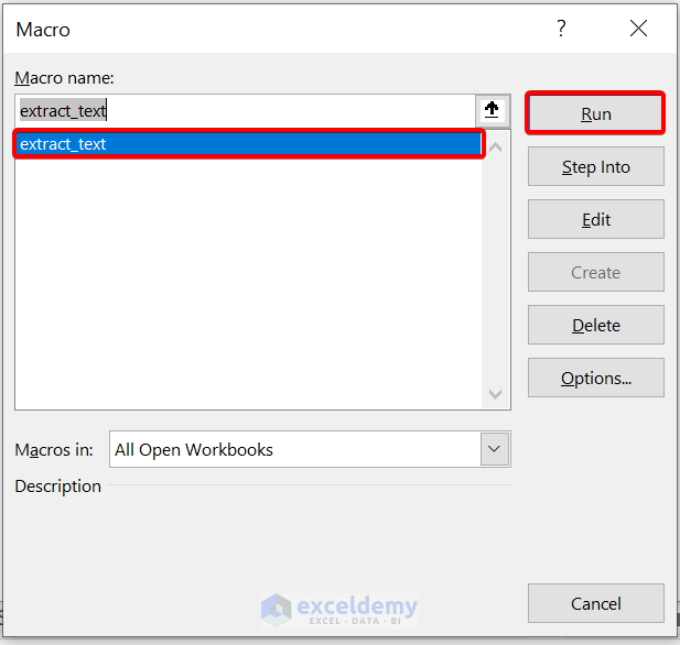
- Click on Run.
Read More: How to Extract Text Between Two Commas in Excel
Things to Remember
✎ If you see a #VALUE! Error, wrap the whole formula under the IFERROR function and create a custom response.
Download the Practice Workbook
Related Articles
- How to Extract Text after Second Comma in Excel
- How to Extract Text between Two Spaces in Excel
- How to Extract Text Between Two Characters in Excel
- How to Extract Certain Text from a Cell in Excel VBA
<< Go Back to Extract Text in Excel | String Manipulation | Learn Excel
Get FREE Advanced Excel Exercises with Solutions!

What if we have same work multiple times in cell, how can we get the word in that case.
Thanks Deep for your excellent and thoughtful question. Let me guide you to fulfill your query.
We can easily extract multiple texts in cells by using different methods of this article but with slight changes.
Suppose you have a dataset where the texts are separated only with hyphens. In this scenario, you should follow the first method in our article. The steps are:
First, arrange the dataset where texts are separated with hyphens.
Second, insert the following formula.
=MID(B5,FIND("-",B5)+1,LEN(B5))Third, after pressing Enter button, you will get the result for this cell.
Last, use the Fill Handle to apply it to all Cells.
But in case, you have emails separated with @ or any other texts separated with special characters then you can use RIGHT, SEARCH & SUBSTITUTE Functions or LEFT, FIND & SUBSTITUTE Functions or RIGHT, REPT & SUBSTITUTE Functions from our article.
Any of these methods will do the work for you. Let me guide you in detail with the steps.
Firstly, you must arrange a dataset where multiple texts are separated with special characters.
Next, use any of the following formulas in the D5 cell(described in our article)
=RIGHT(B5,LEN(B5)-SEARCH("#",SUBSTITUTE(B5,C5,"#",LEN(B5)-LEN(SUBSTITUTE(B5,C5,"")))))or
=SUBSTITUTE(B5,LEFT(B5,FIND(C5,B5)),"")or,
=TRIM(RIGHT(SUBSTITUTE(B5,C5,REPT(" ",LEN(B5))),LEN(B5)))(Note: Please take a glimpse at our main article to understand the insertion of the formula)
Afterward, after pressing Enter button, you will get the result for this cell. You will get the same result for any of the formulas so you can choose any of them.
Last, use the Fill Handle to apply it to all Cells.