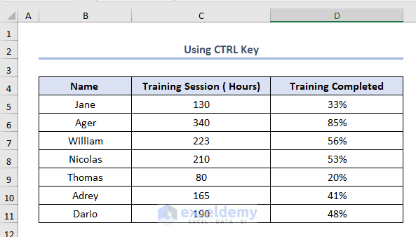
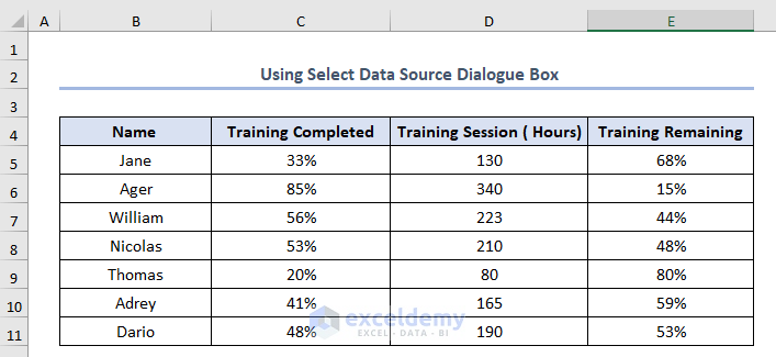
Dataset Overview
We’ve created a dataset called Training Session Dataset for the Year 2021. It features headers labeled as Name, Training Session (Hours), and Training Completed in Columns B, C, and D, respectively. We’ve populated the Training Completed column with values calculated from a total Training Session of 400 hours. Here’s what the dataset looks like.

Method 1 – Using CTRL Key for Selecting Data
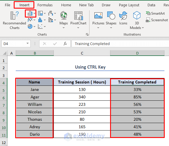
- Select Column B, and while holding the CTRL key, select Column D. This allows you to choose both columns simultaneously.
- Go to the Insert tab and select the Insert Column or Bar Chart option.
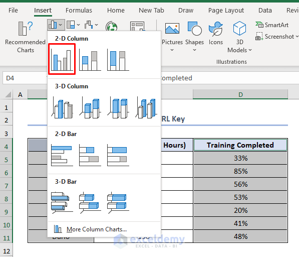
- Choose the 2-D Clustered Column figure.
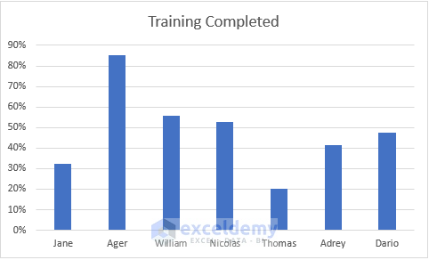
- The resulting chart will display the graphical representation of Training Completed for different individuals.
Method 2 – Utilizing Chart Design Option
- If you have non-adjacent columns, use the Chart Design option.
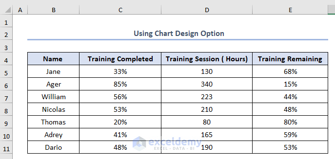
- Add another column (e.g., Column E named Training Remaining) to your dataset.
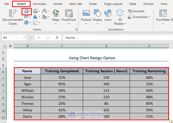
- Select the entire dataset, go to the Insert tab, and choose the Insert Column or Bar Chart option.
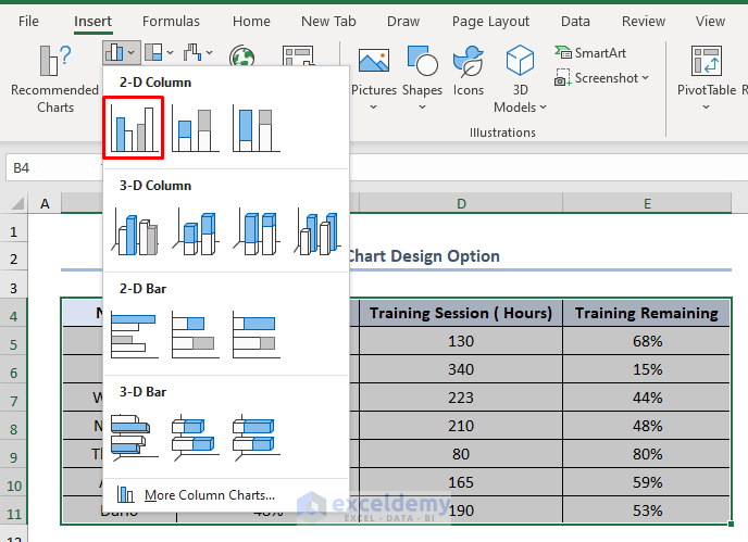
- Select the 2-D Clustered Column option.
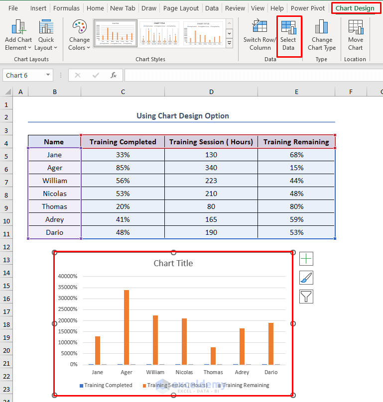
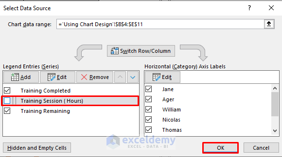
- Click on the chart, go to the Chart Design tab, and choose Select Data.
- In the Select Data Source window, deselect Training Session (Hours).
- Click OK.
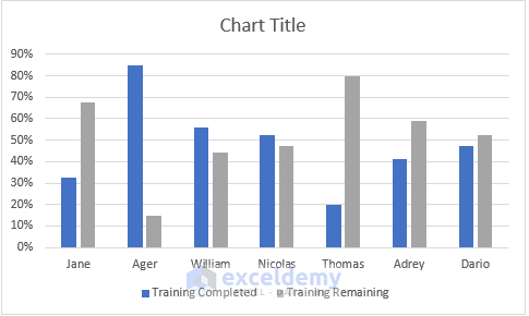
- The chart showing Training Completed and Training Remaining for each person will be displayed.
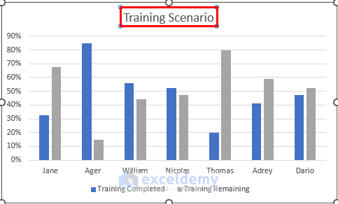
- Edit the chart title to Training Scenario.
Read More: How to Select Data for a Chart in Excel
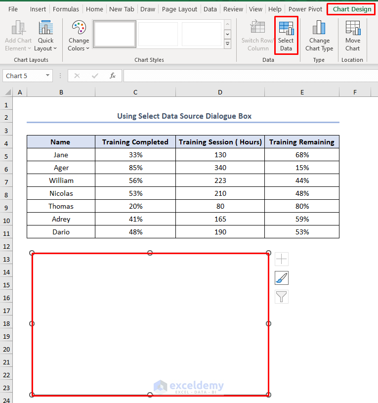
Method 3 – Using Data Source Dialogue Box
- Create a blank chart (similar to Method 2) without selecting the dataset.
- Click on the blank chart, then choose Chart Design and choose Select Data.
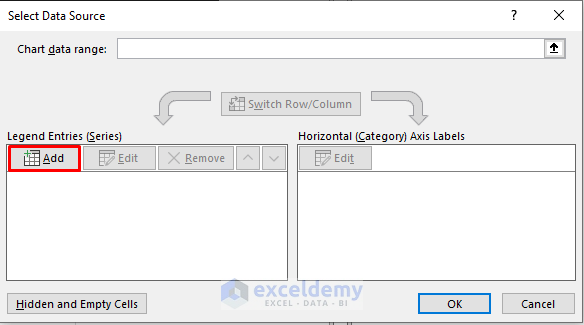
- In the Select Data Source window, click Add.
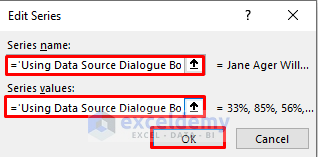
- An Edit Series window will appear. Select cells B5:B11 as the Series Name and C5:C11 as the Series Value.
- Click OK.
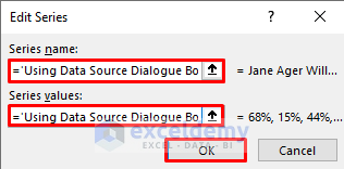
- Again, click Add in the Select Data Source window. Add cells B5:B11 as the Series Name and E5:E11 as the Series Value.
- Click OK.
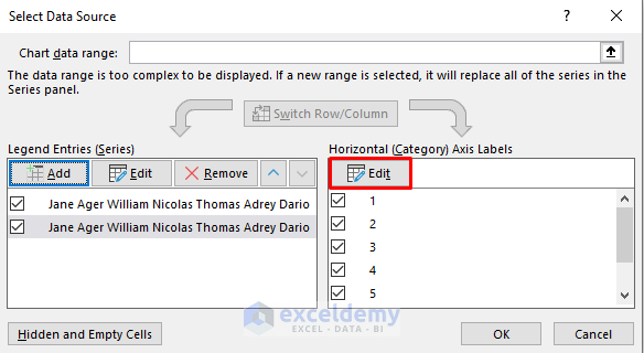
- The Select Data Source window will appear again.
- Click Edit in the Horizontal (Category) Axis Labels bar.
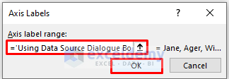
- In the Axis Labels window, add B5:B11 as the axis label range (representing the horizontal axis).
- Click OK.
- Click OK in the Select Data Source window.
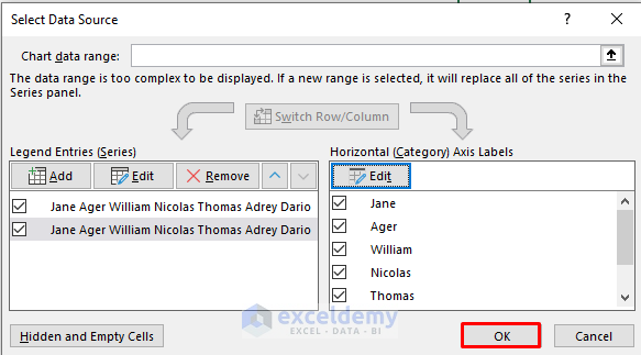
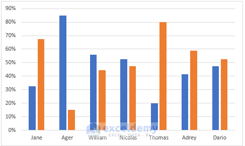
- You’ll get the final chart.
Read More: How to Expand Chart Data Range in Excel
Things to Remember
Remember that in the Edit Series window, you need to add column names in the Series Name bar and column values in the Series Values bar.
Download Practice Workbook
You can download the practice workbook from here:
Related Articles
<< Go Back to Data for Excel Charts | Excel Charts | Learn Excel
Get FREE Advanced Excel Exercises with Solutions!
