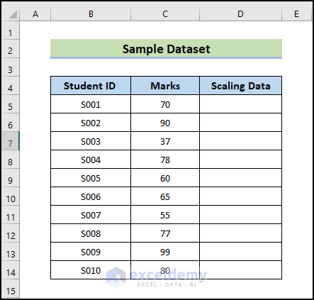
We’ll use the dataset below, which includes student names and corresponding grades. We will scale the data in the Marks column.
Method 1 – Combine MIN and MAX Functions to Scale Data via Min-Max Normalization
Steps:
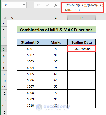
- To scale the Marks column data, use the following formula.
=(C5-MIN(C:C))/(MAX(C:C)-MIN(C:C))
- Press Enter.
- You will get the following scaling data.
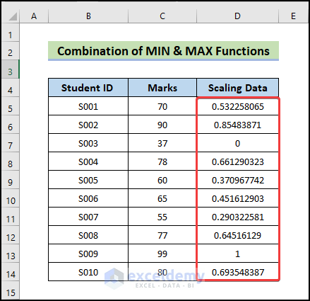
- Drag the Fill Handle icon down to fill the other cells with the formula.
- You will get the scaling data in the entire Marks column.
Note:
- The MIN function does not count blank cells, so it will not return a blank cell if your chosen range of cells includes one. Instead, it will take the least significant value from all other non-empty cells.
- You can input up to 255 arguments into the MIN function.
How Does the Formula Work?
- C5-MIN(C:C): Once the minimum value of the C column has been determined and subtracted from cell C5, the formula C5-MIN(C:C) will return the value of 33.
- (MAX(C:C)-MIN(C:C): This formula will yield the result of 62 after calculating the maximum value of the C column and deducting the minimum value from the maximum value.
- (C5-MIN(C:C))/(MAX(C:C)-MIN(C:C)): The whole formula will return the scale value of 0.532.
Method 2 – Perform Data Scaling Through the Paste Special Feature by Dividing with 100
Steps:
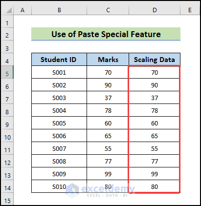
- Copy the data from the Marks column and paste it into the Scaling Data column.
- Enter 100 in any cell outside the dataset and copy it.
- Select the new column made by pasting Marks.
- Right-click on the cell and choose Paste Special from the menu that appears.
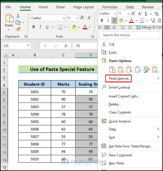
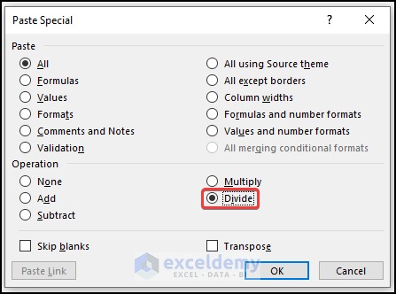
- The Paste Special window will appear.
- Select Divide from the Operation option.
- Click on OK.
- You will receive the Marks column scaling data listed below.
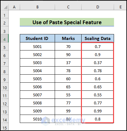
Note that this returns different values than traditional data scaling via min-max normalization.
Read More: How to Scale Data from 1 to 10 in Excel
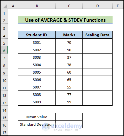
Method – Apply AVERAGE and STDEV Functions
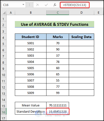
We will scale the data values so that their mean is 0 and their standard deviation is 1. We use the same dataset.
Steps:
- 15 is the mean value, and C16 is the standard deviation value.
- To calculate the mean value, use the following formula.
=AVERAGE(C5:C13)
- Press Enter.
- You will get the following average value.

- To calculate the standard deviation value, use the following formula.
=STDEV(C5:C13)
- Press Enter.
- You will get the following standard deviation value.
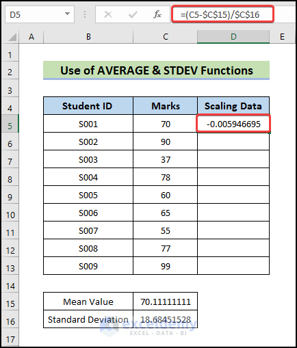
- To calculate the scale data value, select the first cell and use the following formula.
=(C5-$C$15)/$C$16
- Press Enter.
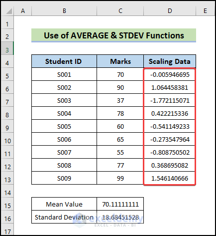
- Dag the Fill Handle icon down to fill the other cells with the formula.
Download the Practice Workbook
<< Go Back to Scaling Formula in Excel | Excel for Statistics | Learn Excel
Get FREE Advanced Excel Exercises with Solutions!
