Need to learn what is page break view in Excel? If you are looking for such unique information, you’ve come to the right place. Here, we will take you through the introduction of the page break view along with 5 easy and convenient methods to activate the page break view in Excel.
What Is Page Break View in Excel?
In Excel, actually, it’s called Page Break Preview instead of page break view. You can see where the page breaks will appear while printing the spreadsheet by using the Page Break Preview option. We use page breaks to separate a worksheet into different pages for printing. Always a visual representation is the best option for better understanding. So, let’s see below.
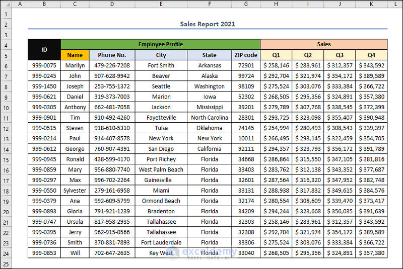
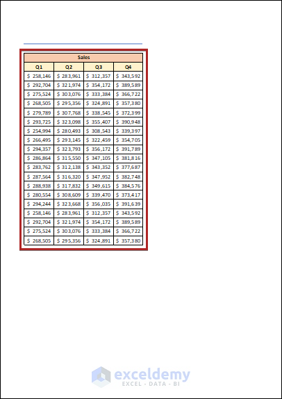
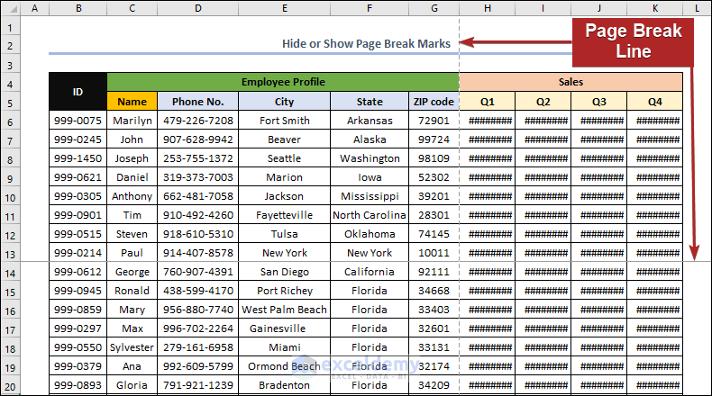
Suppose we have Sales Report 2021 of a certain company. This dataset contains the Employee Profiles and the Quarterly Sales amount of employees.
Now, if we use the Page Break Preview option, the sheet will look like the following one.
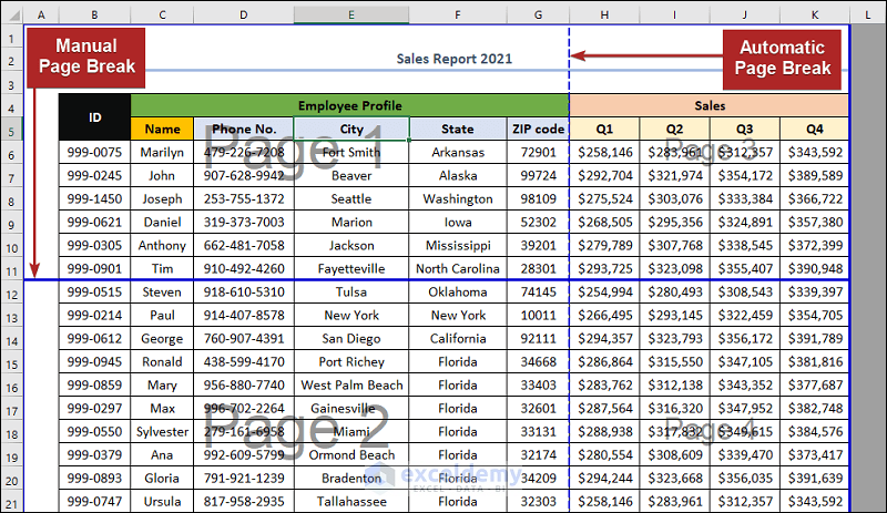
In the picture above, we can see two lines. One is a vertical dashed line, another is a horizontal solid line. These indicate two types of page breaks.
- Automatic Page Break: Excel adds page breaks spontaneously based on the choices for Paper size, Margins, and Scaling. This type of page break is called automatic page break. In the sheet, it reflects itself with a dashed blue line.
- Manual Page Break: If the default page break doesn’t match your printing criteria, you may manually insert a page break with a few easy steps. It’s incredibly handy for printing a range of data with the precise amount of pages you need. This type of page break looks like a solid blue line in the Page Break Preview option.
Activate Page Break View in Excel: 5 Simple Ways
Usually, we see the worksheet in the Normal View by default, which is just like the first image of this article. But, we can see the page break lines in our worksheet with the help of Page Break Preview. Now, we’ll show you five different approaches to activating the Page Break Preview option in Excel. So, without further delay, let’s jump into the methods one by one.
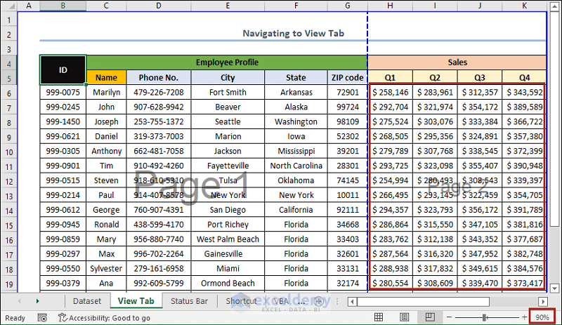
1. Navigating to View Tab
In our first method, we’ll get help from the View tab. Follow the steps below.
📌 Steps
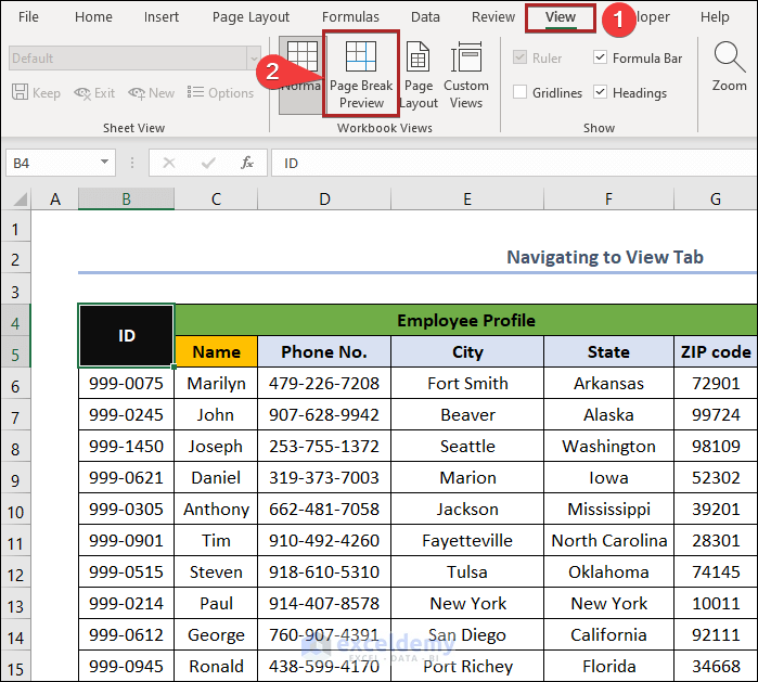
- At first, navigate to the View tab.
- Then, select the Page Break Preview from the Workbook Views group on the ribbon.
At this moment, we’re watching the sheet in page break view mode. We clearly can see the sheet divided into two portions by a dashed blue line. It stands for the two portions to be printed on two different pages. Obviously, you can see Page 1 and Page 2 appear as watermarks on the respective pages. These are the corresponding page numbers.
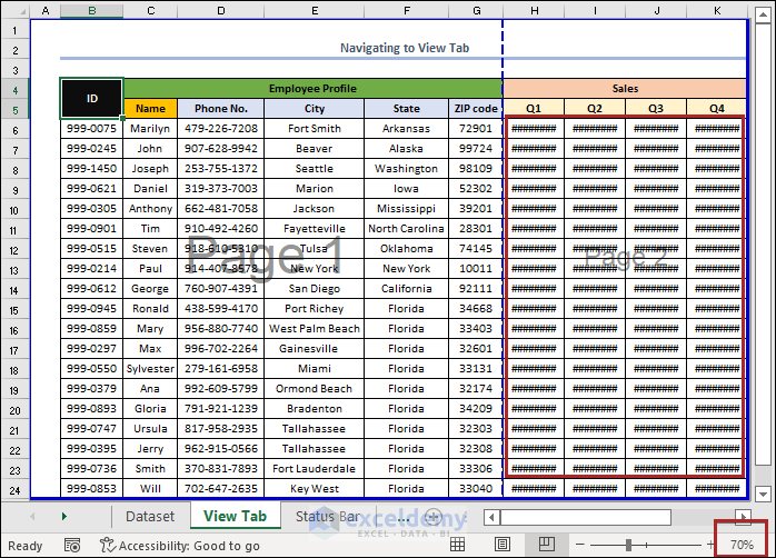
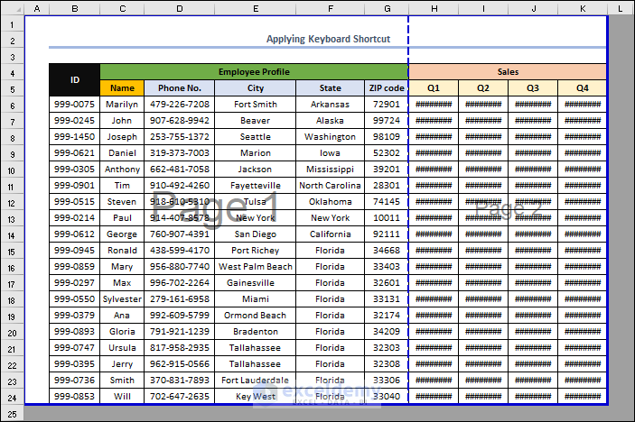
Note: The Sales amounts aren’t showing in cells in the H6:K24 range. Because the application of Page Break Preview automatically sets the Zoom level to 70%. So, the digits cannot capacitate themselves into the cells. As a result, they are shown with hash (#) signs.
- Now, set the Zoom level at 90% and you can see those numbers also.
2. Using Status Bar to Activate Page Break View in Excel
The second method reflects the usage of the Status Bar. Follow the steps carefully.
📌 Steps
- Firstly, go to the Status Bar at the bottom of the window.
- Secondly, select the Page Break Preview button at the left of the Zoom Level option.

Instantly, you can see the worksheet Status Bar shown in page break view mode.

3. Applying Keyboard Shortcut
In this instance, I’m aware of your thoughts. Do shortcut keys exist? You’re lucky! Yes, shortcut keys exist to do this job more quickly. Follow the steps carefully.
📌 Steps
- Firstly, press the ALT key followed by W and I on your keyboard.
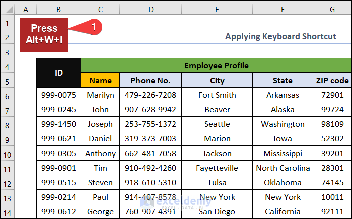
- Then, magically you can see the worksheet in the Page Break Preview mode.
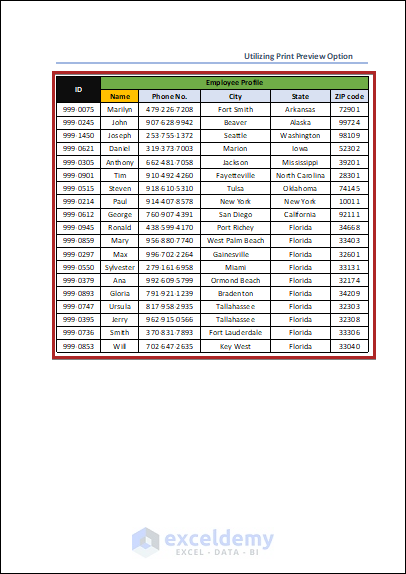
4. Utilizing Print Preview Option
In some situations, you can see the page break utilizing the Print Preview in Excel. The distinction between viewing page breaks in Print Preview and Page Break Preview isn’t too much. You will be able to comprehend the allocation page by page while seeing page breaks in the Print Preview option. But viewing in Page Break Preview allows you to see the whole distribution In this mode, you can see all of the pages and page breaks in the display. Now, follow the steps below.
📌 Steps
- At the very beginning, press CTRL+P on your keyboard.

Hence, you can see where the page break will happen while printing.
5. Employing VBA Code
Employing the VBA code is always an amazing alternative. Follow the steps below to be able to solve the problem in this way.
📌 Steps
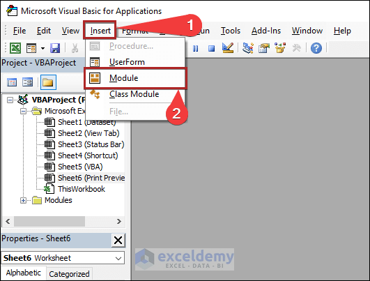
- Firstly, press the ALT+F11 key.

- Suddenly, the Microsoft Visual Basic for Applications window will open.
- Then, go to the Insert tab.
- After that, select Module from the options.
- It opens the code module where you need to paste the code below.
Sheet5.Activate
ActiveWindow.View = xlPageBreakPreview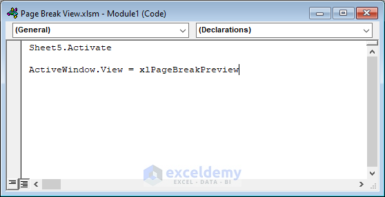
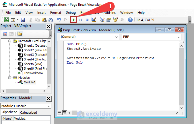
- Then click on the Run button or press the F5 key on your keyboard.
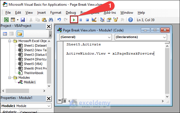
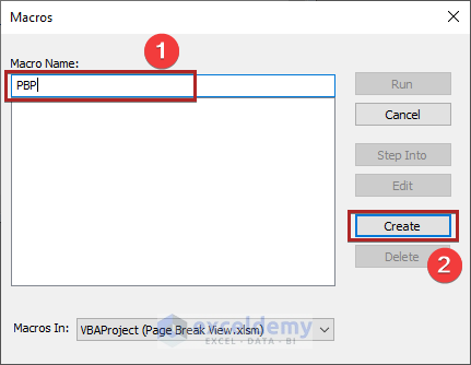
- Eventually, the Macros dialog box will open.
- At this moment, write down a name in the Macro Name box. In this case, we named the macro PBP (Page Break Preview).
- Then, click on the Create button.
In this instance, you can see the below code in the code module.
Sub PBP()
Sheet5.Activate
ActiveWindow.View = xlPageBreakPreview
End Sub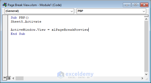
- Again, select the Run button.
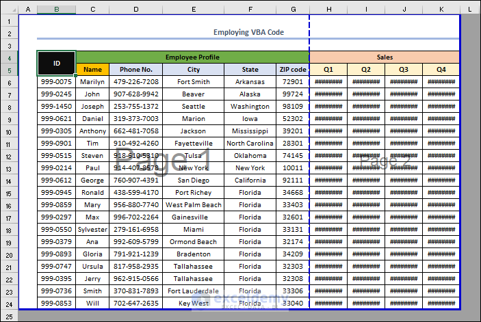
Instantly, the worksheet VBA looks like the one below.
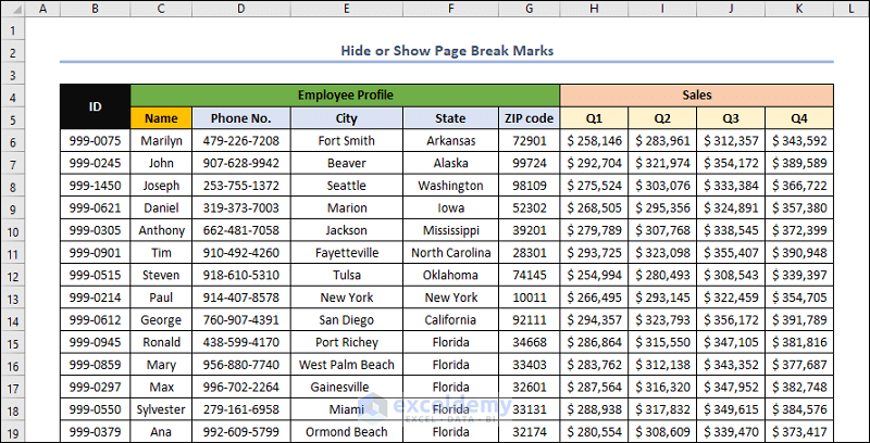
How to Hide or Show Page Break Marks in Excel
If we change the view to Page Break Preview once, we can see these kinds of lines in the Normal view also.
Sometimes, it becomes very annoying to see these lines while working on the sheet.
To solve this problem, we can hide the page break lines. Again, we can activate the option to show them as per our preference. Follow the steps below.
📌 Steps
- Firstly, move to the File tab.
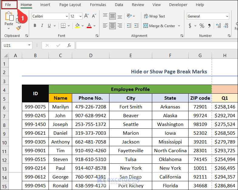
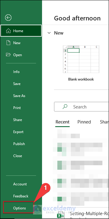
- Secondly, select Options as shown in the image below.
- Hence, the Excel Options window opens.
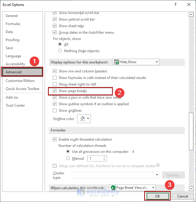
- Then, go to the Advanced tab.
- After that, uncheck the box of Show page breaks under the section of Display options for this worksheet.
- Finally, click OK.
Now, we can’t see any page break lines in our worksheet.
Again, we can show the page break lines repeating the same steps.
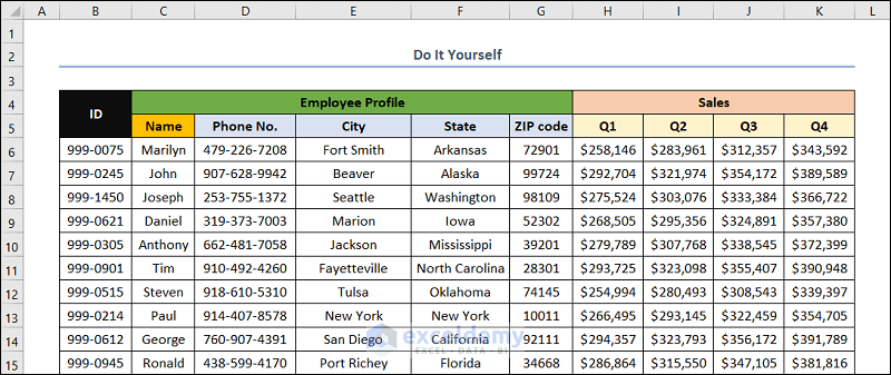
Practice Section
For doing practice by yourself we have provided a Practice section like below in the last sheet named Practice Section on the workbook. Please do it by yourself.
Download Practice Workbook
You may download the following Excel workbook for better understanding and practice yourself.
Conclusion
This article provides a brief description of Page Break Preview and how to activate it in Excel. Don’t forget to download the Practice file. Thank you for reading this article, we hope this was helpful. Please let us know in the comment section if you have any queries or suggestions.
Related Articles
- How to Show Only One Page in Excel Page Layout View
- How to Show Ruler in Excel
- [Fixed!] Excel Ruler Not Showing
- What Is Page Layout View in Excel?
- What Is Datasheet View in Excel?
<< Go Back to Workbook Views | Workbook in Excel | Learn Excel
Get FREE Advanced Excel Exercises with Solutions!
