How to Use a Data Model in Excel – 3 Examples

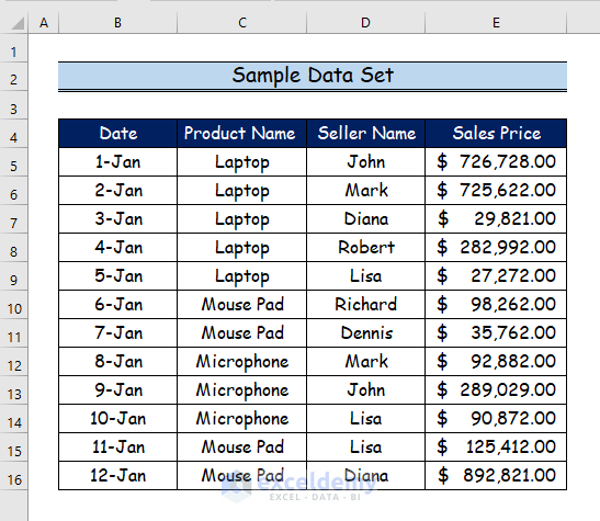
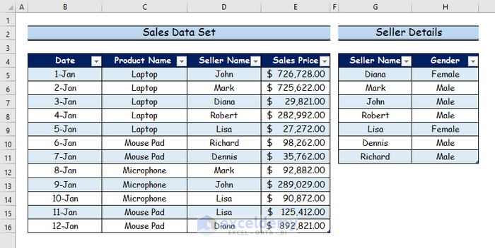
The sample dataset includes sales price, seller name, product name, and date. There’s another dataset that contains the seller’s name and gender.

Example 1 – Convert the Datasets to Table Objects

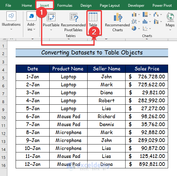
Step 1:

• Click the data set.
• Go to the Insert tab.
• Choose Table.

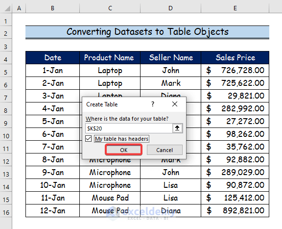
Step 2:

• Click OK.

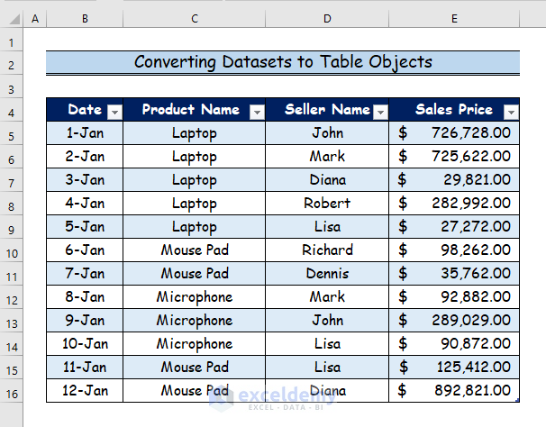
Step 3:

The dataset is converted into a table.

Read More: How to Create a Data Model in Excel

Example 2 – Using the Power Pivot to Add a Table to a Data Model to Create Relationships

Step 1:

The two datasets are converted to a table.

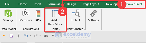
Step 2:

• Select Power Pivot.
• Choose Add to Data Model Tables.

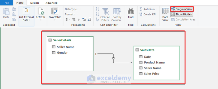
Step 3:

• To view the connections between the two data tables, select Diagram View.

Read More: Excel Data Model vs. Power Query: Main Dissimilarities to Know

Example 3 – Creating a Pivot Table

Step 1:

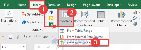
• Go to the Insert tab.
• Choose Pivot Table.
• Select “From Data Model”.

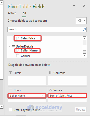
Step 2:

• Drag Seller Name to Rows and Sales Price to Values.

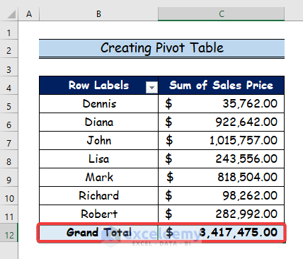
Step 3:

This is the output.

Read More: How to Add Table to Data Model in Excel

Download Practice Workbook

Download the Excel workbook.

Related Articles

• How to Get Data from Data Model in Excel
• How to Remove Table from Data Model in Excel
• How to Update Data Model in Excel
• How to Use Reference of Data Model in Excel Formula

<< Go Back to Data Model in Excel | Learn Excel