How to Shuffle Numbers in Excel (7 Easy Methods)

Excel can help you shuffle or randomize different formats of data quickly in easy ways. You can shuffle data within one column as well as around different columns. In this article, we will show you how to shuffle numbers in Excel in 7 easy methods.

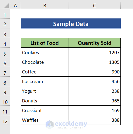
In this article, we will demonstrate how to shuffle numbers in Excel in 7 effective ways. We will use the following dataset for this purpose.

1. Inserting RAND Function

This is one of the easiest methods to shuffle data in Excel. Follow these steps to learn how to use the RAND function to shuffle numbers.

Steps:

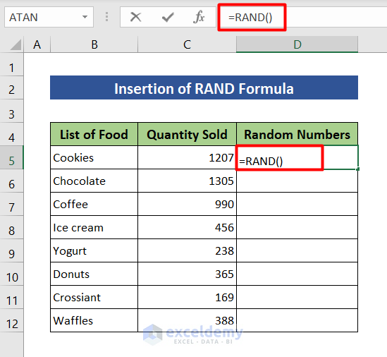
• First of all, insert a column of Random Numbers and type the following formula.

• RAND() returns any evenly distributed random real number greater than or equal to 0 and less than 1.

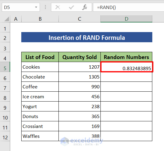
• Next, press Enter to get the random number in cell D5.

• Now, double-click at the bottom right corner of cell D5 to copy the formula to all cells.

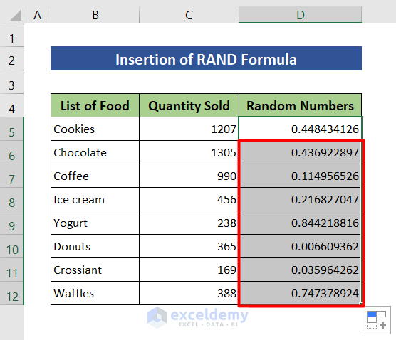
• Once you get the random numbers in the whole column, select all the random numbers and go to the DATA tab.

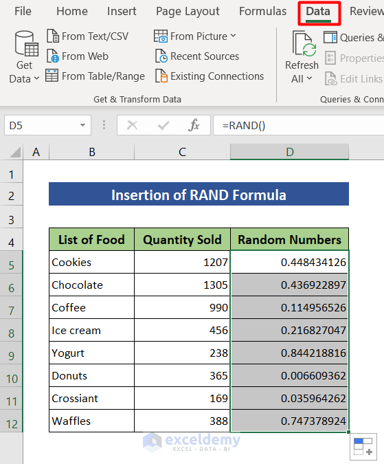
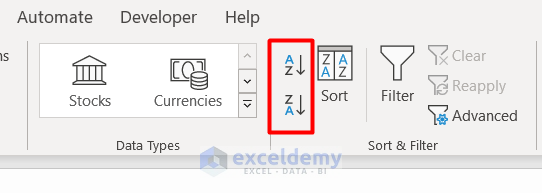
• Then select either Sort Smallest to Largest or Sort Largest to Smallest from the Sort & Filter settings.

• Once you select one of the two options, a pop-up box will appear.
• Click on Expand the selection and press Sort.

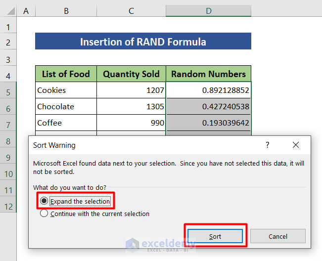
• The List of Food and Quantity Sold will be shuffled.

Read More: How to Randomize a List in Excel Without Duplicates (4 Ways)

2. Applying RANDBETWEEN Function

We will use the RANDBETWEEN function to shuffle numbers in columns now. The steps are discussed below.

Steps:

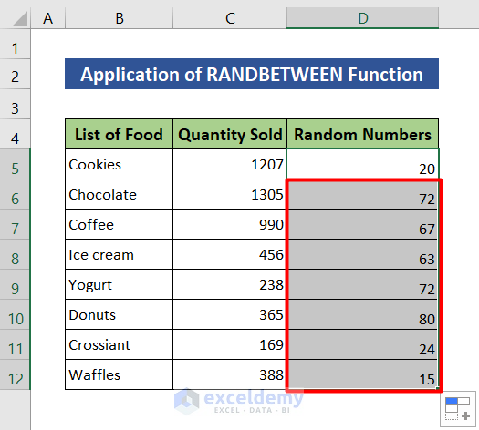
• First, insert a column of Random Numbers, and then write down the following formula in cell D5.

• RANDBETWEEN function returns random integer numbers between a specified range. (1,100) refers to the range. Selecting a smaller range can return the same value for more than one cell. The larger the range, the lower the chance of repetition. Therefore, choose a large range to avoid repetition.

• Now, press Enter to get a random value between 1 to 100 in cell D5.

• Next, move your cursor to the bottom right corner of cell D5 and click twice.
• All cells will be filled with random numbers between 1 to 100.

• Now, select all the random numbers and press Alt+A+SA to sort the values from smallest to largest.
• A pop-up window will show up. Just select Expand the selection and click on Sort.

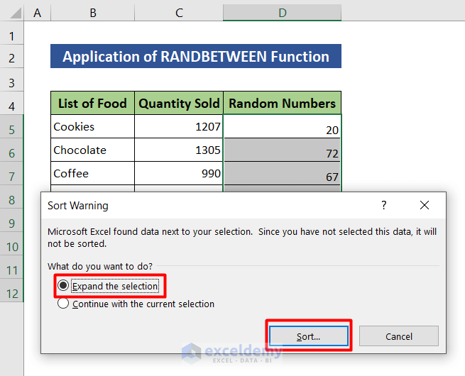
• All the data of columns B and C will be randomized and you will get your desired results.

Read More: How to Randomize List of Names in Excel (8 Easy Methods)

3. Combining SORTBY and RANDARRAY Functions

In this method, we will shuffle numbers in Excel by combining the SORTBY function and the RANDARRAY function. Keep on reading to learn how to do it.

Steps:

• Initially, insert a new column (Random Numbers) to generate random numbers.
• Then type the following formula in cell D5.

• RANDARRAY returns an array of random numbers. “8” refers to the number of rows with data and “1” refers to the number of columns.

• Hit the Enter button and then double-click the bottom right corner of cell D5.

• Now we want to shuffle the numbers in the Quantity Sold To do that, write down the formula given below.

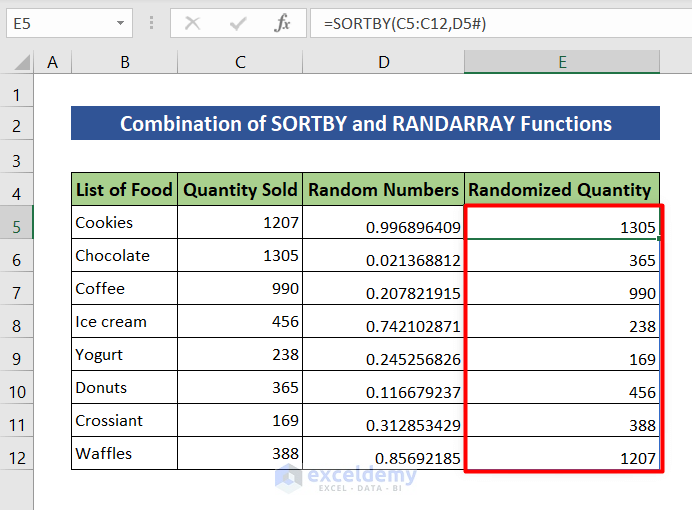
• SORTBY sorts the contents of a range or array based on the values in a corresponding range or array. C5:C12 refers to cells C5 through C12. D5# refers to the random values of column D based on which the sorting will be done.

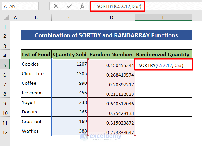
• Press the Enter button.
• To copy the formula to all the cells, click two times at the bottom right corner of cell E5.
• Thus you will get the shuffled numbers.

Read More: How to Shuffle an Array Using Excel VBA (4 Examples)

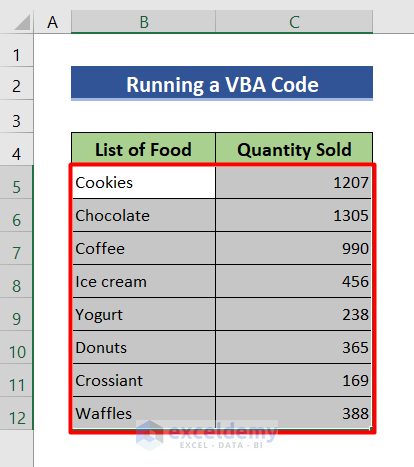
4. Running a VBA Code

Now we will run a VBA code to shuffle data in Excel. The VBA code given in this method can shuffle data from one column to another. We will show you how you can apply this VBA code in your Excel.

Steps:

• First, select all the data you want to shuffle.

• Next, press Alt+F11 to open Microsoft Visual Basic window.

• Then click on the Insert tab in that window and select Module.

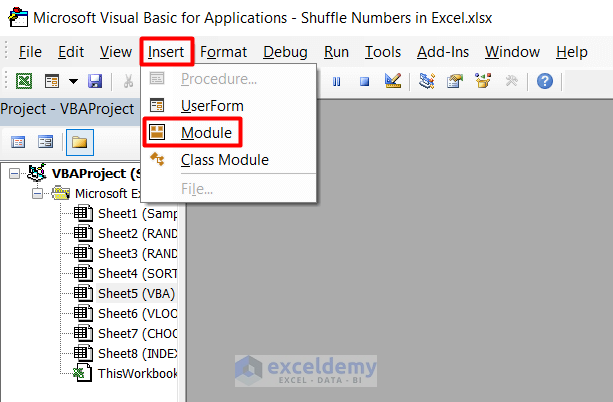
• A module to write codes will open. Copy the following VBA code in the module.

Sub Shuffle()
  Dim range As range
  Set range = Selection

  Dim Row As Long
  Dim Column As Long

  Row = range.Columns.Count
  Column = range.Rows.Count

  Dim i As Long
  Dim j As Long
  For i = Column To 1 Step -1
    For j = Row To 1 Step -1
      Dim rndRow As Long
      Dim rndColumn As Long
      rndRow = Application.WorksheetFunction.RoundDown(Column * Rnd + 1, 0)
      rndColumn = Application.WorksheetFunction.RoundDown(Row * Rnd + 1, 0)

      Dim temp As String
      Dim tempColor As Long
      Dim tempFontColor As Long

      temp = range.Cells(i, j).Formula
      tempColor = range.Cells(i, j).Interior.Color
      tempFontColor = range.Cells(i, j).Font.Color

      range.Cells(i, j).Formula = range.Cells(rndRow, rndColumn).Formula
      range.Cells(i, j).Interior.Color = range.Cells(rndRow, rndColumn).Interior.Color
      range.Cells(i, j).Font.Color = range.Cells(rndRow, rndColumn).Font.Color

      range.Cells(rndRow, rndColumn).Formula = temp
      range.Cells(rndRow, rndColumn).Interior.Color = tempColor
      range.Cells(rndRow, rndColumn).Font.Color = tempFontColor
    Next j
  Next i

End Sub

• Now press F5 to run the code.
• Go back to the worksheet and you will find all that all the data are shuffled.

5. Combining VLOOKUP and RANDBETWEEN Functions

In this method, we will combine the VLOOKUP function and the RANDBETWEEN function to shuffle numbers in Excel. Read the following steps to do it.

Steps:

• First of all, insert a column named Random Numbers and type the following formula to generate random numbers.

• (1,8) refers to any number between 1 to 8 that the RANDBETWEEN function will return.

• Hit Enter and double-click the bottom right corner of cell D5 to copy the formula to all the cells.

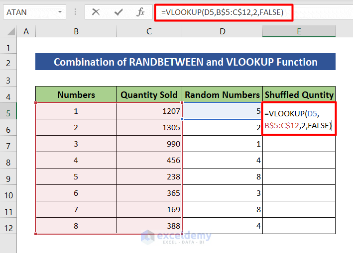
• Now to get the shuffled value of column C, type the following formula in cell E5.

• D5 refers to the first value of the random numbers. B$5:C$12 is an absolute reference to the cells B5 through C12. FALSE refers to the exact match.

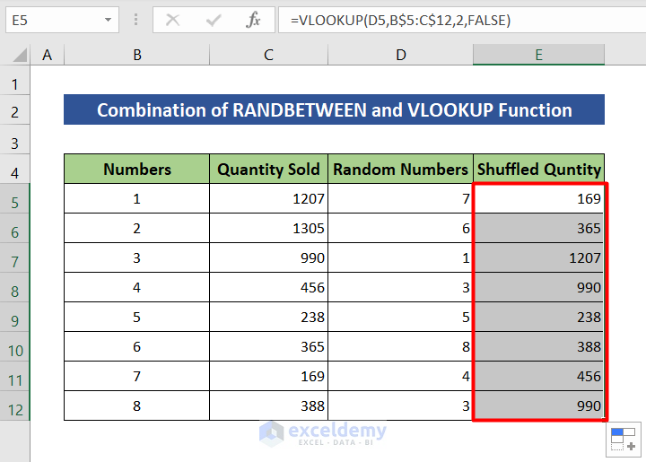
• Press Enter.
• Now copy the formula to all the cells by clicking twice at the bottom right corner of cell E5 and there you have your shuffled quantity.

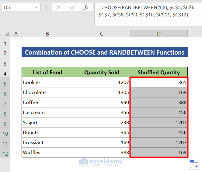
6. Merging CHOOSE and RANDBETWEEN Functions

In this part of the article, we will shuffle numbers in Excel by merging the CHOOSE function and the RANDBETWEEN function.

Steps:

• First, insert a new column ( Shuffled Quantity) and write down the following formula in cell D5.

• $C$5, $C$6,$C$7, $C$8, $C$9, $C$10, $C$11, $C$12 refers to the values of C5 to C12.

• Hit Enter on your keyboard and left-click the bottom right corner of cell D5 twice.
• You will find the desired results in D column.

Read More: How to Randomize a List in Excel Into Groups (5 Suitable Ways)

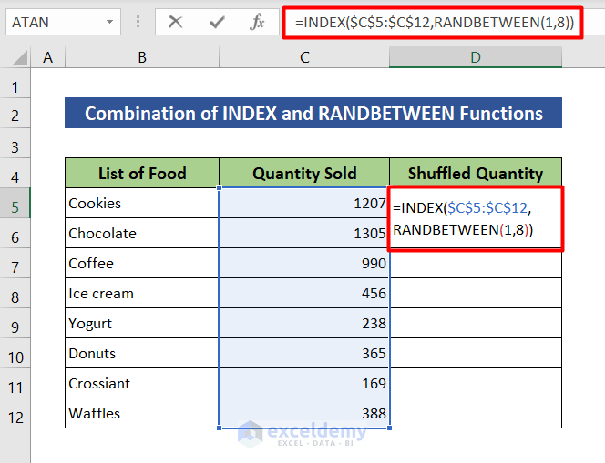
7. Merging INDEX and RANDBETWEEN Functions

Before conclusion, we will see one last method to shuffle numbers in Excel. We will use the INDEX function and the RANDBETWEEN function for this purpose. The procedure is discussed below:

Steps:

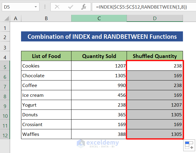
• First of all, write down the formula given below in your desired cell.

• $C$5:$C$12 refers to the cells from C5 to C12.

• Hit Enter and copy the formula by double-clicking the bottom right corner of cell D5 to get the desired results.

Things to Remember

• If you want to shuffle values around different columns, use the VBA code. Other methods shuffle values within the same column only.
• Don’t forget to give proper cell references or you won’t get the desired results.
• Input a large range in the RANDBETWEEN function to avoid repetition of the same numbers.

Download Practice Workbook

Download this practice workbook for practice while you are reading this article.

Concluding Remarks

Thanks for making it this far. I hope you find this article useful. Now you know 7 different methods to shuffle numbers in Excel. Please let us know if you have any further queries and feel free to give us any recommendations in the comment section below.

Related Articles

• How to Do Factorials in Excel (6 Easy Methods)