How to Hide Columns in Excel (6 Easy Ways)

Method 1 – Using the Home Tab from the Ribbon

• Select the column(s) you want to hide.
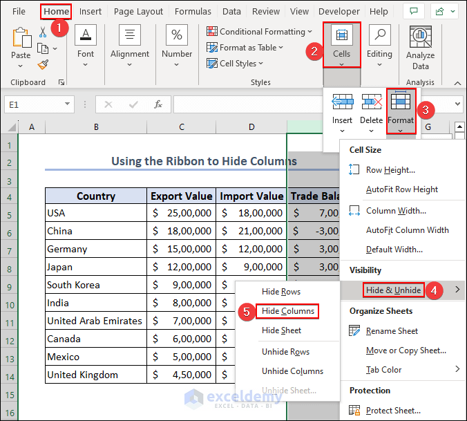
• Navigate to the Home tab on the ribbon.
• Go to the Cells group.
• Click on the Format button.
• Choose Hide & Unhide and select Hide Columns.

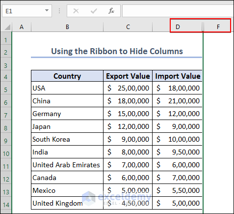
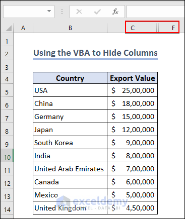
• We have hidden column E. In the image, columns D and F are displayed but not column E.

Method 2 – Using the Context Menu to Hide Columns in Excel

• Select columns (for example, column E).\
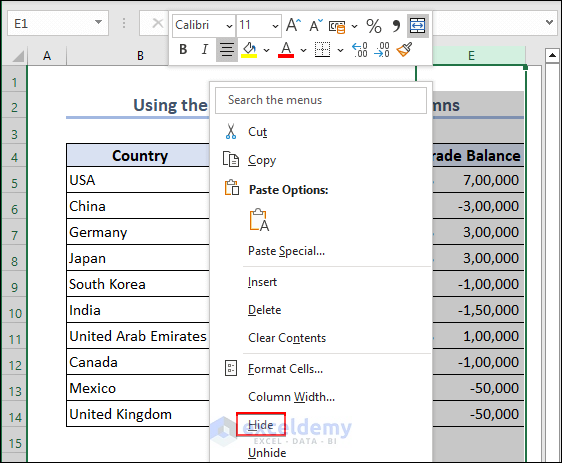
• Right-click on the column header(s) you wish to hide.
• From the context menu, select Hide.

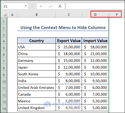
• We have hidden column E. In the image, columns D and F are displayed but not column E.

Method 3 – Using the Keyboard Shortcut to Hide Columns

• Select the column(s) you want to hide.
• Press Ctrl + 0.
• The selected columns will be hidden instantly.

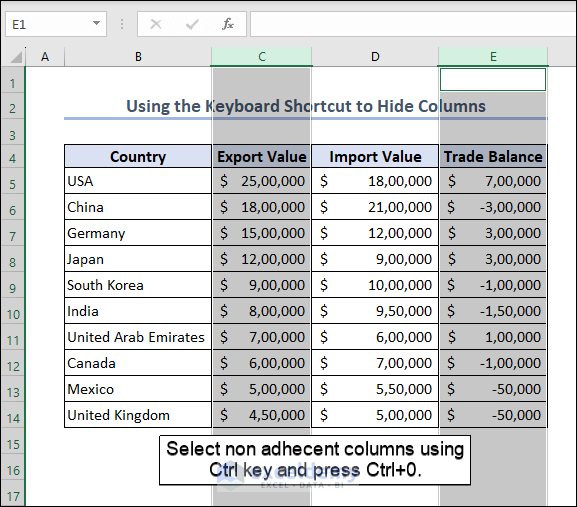
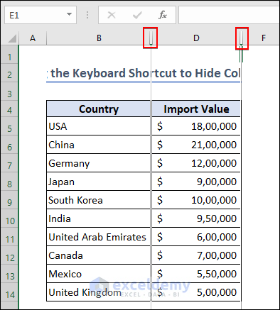
• You will see a small gap where a column between adjacent columns is hidden. Column C is hidden, so there is a small gap between Column B and Column D.

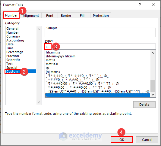
Method 4 – Using the Format Dialog Box to Hide Columns in Excel

• Select the column(s) you want to hide.
• Right-click and select Format Cells.
• Alternatively, press the Ctrl + 1 to open the Format Cells dialog box.

• In the dialog box, navigate to Number.
• Select Custom.
• Enter ;;; in the Type box.
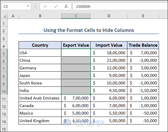
• Press OK to hide the selected cells.

• The selected cells are hidden in a column.

Method 5 – Using the Data Tab from the Ribbon to Hide Columns

• Select columns.
• Go to Data tab and pick Group.
• Click the minus(–) sign to hide the columns.

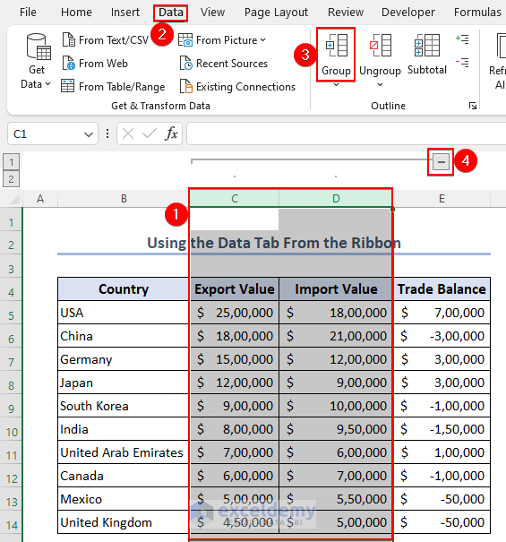
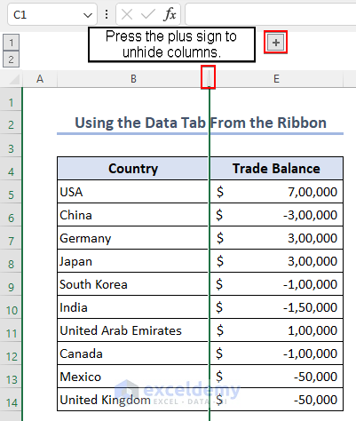
• Columns C and D are hidden. You can click the plus sign, to unhide the columns.

Read More:

• Hide and Unhide Columns in Excel
• Hide Extra Columns in Excel
• Unhide Columns in Excel
• Unhide Columns in Excel All at Once

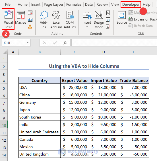
Method 6 – Using VBA Macro to Hide Columns

• Go to the Developer tab and select Visual Basic. 

• Enter the following VBA code to hide column D and column E:

Sub Hide_the_Columns()
Columns("D:E").Hidden = True
End Sub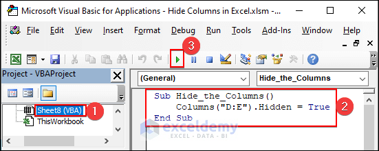

• Now columns D and E are not displayed in Excel.

Read More:

• Hide Columns with Button in Excel
• Hide Columns with No Data in Excel
• Hide Multiple Columns in Excel
• Hide Columns Without Right Click in Excel

How to Unhide Hidden Columns

Method 1 – Using Context Menu

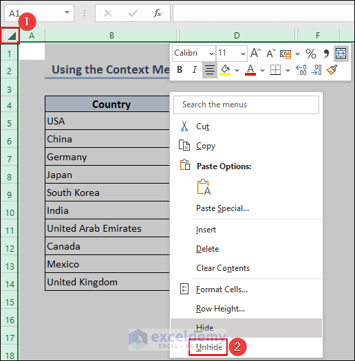
• Select the top left corner of your worksheet.
• Right-click on any column header.
• Select Unhide.

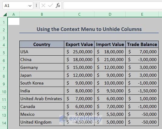
• Now in the following image, we can see all the columns.

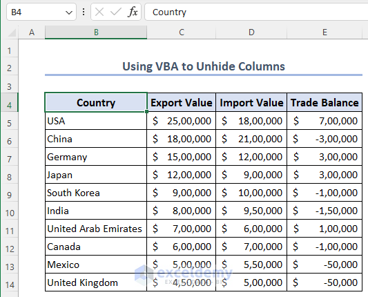
Method 2: Using VBA to Unhide Columns

• Enter the following VBA code to unhide any columns:

Sub Unhide_Columns_in_Whole_Workbook()
Dim x As Worksheet
For Each x In Worksheets
x.Columns.EntireColumn.Hidden = False
Next x
End Sub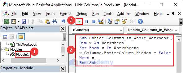

• Here is the final image of Using VBA to Unhide Columns.

Read More:

• Unhide Columns Is Not Working in Excel
• Unhide Columns in Excel Shortcut Not Working
• Hide Columns in Excel with Minus or Plus Sign

Things to Remember

Column Dependencies: Before hiding a column, ensure that it does not contain important data or formulas that are used in other parts of your worksheet. Hiding a column can affect calculations or references in your workbook.

Print Considerations: When preparing your worksheet for printing, remember that hidden columns may still be included in the printed output. Adjust the print settings accordingly to exclude hidden columns if needed.

Data Integrity: Hiding columns does not protect or secure the data within them. If you have sensitive information, consider using other methods, such as data protection or password encryption, to safeguard your data.

Frequently Asked Questions (FAQs)

1. Can hidden columns still be referenced in formulas?

Yes, hidden columns can still be referenced in formulas. Formulas that refer to hidden columns will continue to calculate as normal. However, it’s important to ensure that the hidden column’s data is not critical for the formula’s accuracy.

2. Can hidden columns be seen by others who access my Excel file?

Yes, anyone with access to the Excel file can unhide the hidden columns. Hiding columns in Excel is not a security measure to protect sensitive information. If you need to secure data, consider using other methods like password protection or encryption.

3. How can I unhide columns in Excel?

To unhide columns, select the columns on either side of the hidden columns, right-click, and choose the “Unhide” option from the context menu. You can also use the “Format” option in the “Cells” group on the ribbon to unhide columns.

Download Practice Workbook

You can download the practice workbook from the following download button.

How to Hide Columns in Excel: Knowledge Hub

• Group and Hide Columns in Excel
• Collapse Columns in Excel
• Hide Columns Based on Cell Value without Macro

<< Go Back to Learn Excel