This tutorial will illustrate how to find Chi-Square critical values in Excel. Suppose we will perform a Chi-Square test. As a result, we will get a test statistic. Basically, we use the Chi-Square critical value to check whether the results of the Chi-Square test are statistically significant or not. The test findings are statistically significant if the test statistic is larger than the Chi-Square critical value. So, let’s start the discussion by finding Chi-Square critical value.
How to Find Chi-Square Critical Value in Excel: 2 Quick Tricks
Throughout this article, we will see 2 quick tricks to find Chi-Square critical value in Excel. To find the Chi-Square critical value we need to know two values.
- Level of significance.
- Degrees of freedom.
We can use these two values to figure out the Chi-Square critical value. Also, we can compare this value with the test statistics.
1. Use CHISQ.INV.IRT Function to Find Chi-Square Critical Value
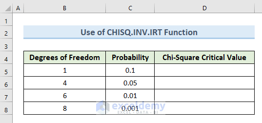
In the first method, we will use the CHISQ.INV.IRT function to find the Chi-Square critical value in Excel. The CHISQ.INV.IRT function in Excel enumerates the critical value of the Chi-Squared distribution. To illustrate this method we will use the following dataset. In the dataset, we have some Degrees of Freedom and Probability values. Using the CHISQ.INV.IRT function we will find the Chi-Square critical value.
Let’s see the steps to implement this method.
STEPS:
- To begin with, select cell D5.
- In addition, type the following formula in that cell:
=CHISQ.INV.RT(C5,B5)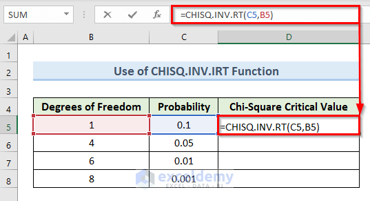
- Press Enter.
- As a result, we get a Chi-Square critical value in cell D5.

- Furthermore, drag the Fill Handle tool from cell D5 to D8.
- Lastly, we can see the results in the following image.

Limitations of CHISQ.INV.RT Function in Excel
- The value of Probability and ‘degree of freedom’ in the INV.RT function has to be a number. Otherwise, that function will return the #VALUE error.
- The CHISQ.INV.RT function will return #NUM error:
- If the value of probability is larger than 1 or less than 0.
- If the value of the ‘degree of freedom’ is less than 1 or larger than 0.
- The CHISQ.INV.RT function only accepts integer values of the ‘degree of freedom’ argument. If we input a non-integer value, the function will only consider the integer part. For example, we will get the same value if we input the values 4, 4.5, and 4.2 as degrees of freedom.
2. Find Chi-Square Critical Value for Earlier Excel Versions with CHISQ.INV Function
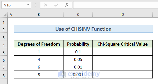
If you are using Excel 2007 and earlier versions of Excel the CHISQ.INV.RT function is not available there. In the earlier versions, we have to use the CHISQ.INV function instead of the CHISQ.INV.RT function. The main purpose of the above two functions is the same. The CHISQ.INV.RT function is just the updated version of the CHISQ.INV function. To demonstrate the use of this function we will use the following dataset.
Let’s see the steps to perform this action.
STEPS:
- Firstly, select cell D5.
- Secondly, insert the following formula in that cell:
=CHIINV(C5,B5)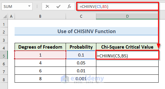
- Press Enter.
- So, we get the value of Chi-Square critical value in cell D5.

- After that, drag the Fill Handle tool from cell D5 to D8.
- Finally, we get our desired Chi-Square critical values like the following image.

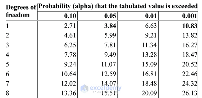
Utilize Chi-Square Distribution Table
We can also find the Chi-Square critical value with the Chi-Square distribution table. In the following image, we have the Chi-Square distribution table. From the table, we can find critical values for various probability levels and degrees of freedom.
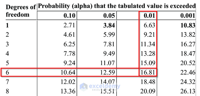
Suppose we want to find the critical value for a probability level of 0.01 and degree of freedom = 6. So, in the distribution table find the intersection point of the row and column that contains the values 6 and 0.01 respectively. In the following image, we can see that the critical value is 16.81.
Read More: How to Find Z Critical Value in Excel
Download Practice Workbook
You can download the practice workbook from here.
Conclusion
In conclusion, this tutorial demonstrates 3 quick tricks to find Chi-Square critical value in Excel. Download the practice worksheet contained in this article to put your skills to the test. If you have any questions, please leave a comment in the box below. Our team will try to respond to your message as soon as possible. Keep an eye out for more inventive Microsoft Excel solutions in the future.
Related Articles
- How to Find T Critical Value in Excel
- How to Find F Critical Value in Excel
- How to Find Critical Value of r in Excel
- Find Critical Value in Excel
<< Go Back to Critical Value in Excel | Excel for Statistics | Learn Excel
Get FREE Advanced Excel Exercises with Solutions!
