Excel Auto Fit Row Height for Wrap Text (4 Methods)

This article illustrates 4 different methods on how to auto-fit row height and column width of cells for wrap text in Excel. Following this article might be a great help for you if you often work with wrapped texts in Excel. Have a quick look through this article to learn how to do that quickly and save a lot of your time and effort. The following picture highlights the purpose of this article.

Excel Auto Fit Row Height for Wrap Text: 4 Ways

Here I am going to highlight the methods for you. So let’s begin.

1.  Use Keyboard Shortcuts to Auto Fit Row Height of Wrap Text in Excel

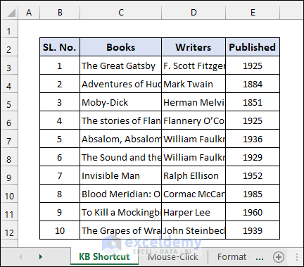
• Imagine you have copied some data from a source and pasted it on your worksheet as follows. The data contains the list of top ten books by American authors.

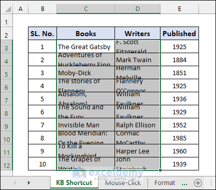
• Now, to apply Wrap Text using a Keyboard shortcut, select the entire range of data. After that, press ALT+H+W. Then the data will look like the below.

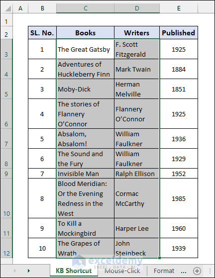
• We have not got the desired result yet. Because the row heights of the cells containing wrap texts do not fit properly. To fix this issue, hold the Alt key and then press H, O, and A successively. Then you will see the following result.

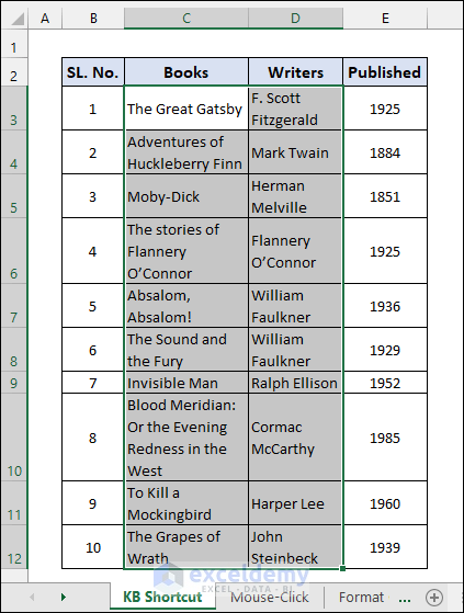
• After that, you can press ALT+H+O+I to auto-fit the column widths.

2. Auto Fit Row Height of Wrap Text with Mouse-Click

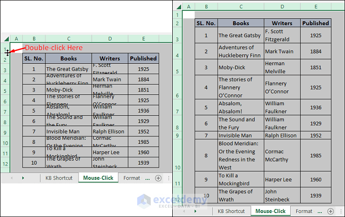
• You can also do that with just a double-click on the row separator line. First press CTRL+A+A to select the entire worksheet. Then put the mouse on the line separating the row numbers as shown below. Next, double-click on it. After that, the row heights will adjust automatically.

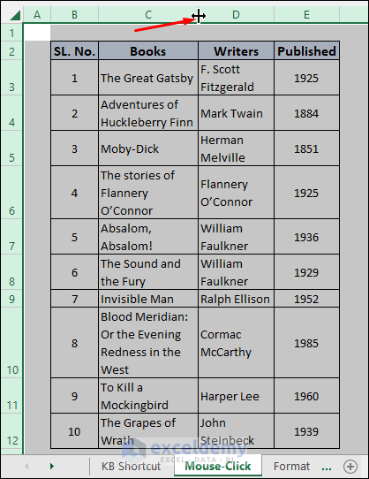
• You can also double-click on the line separating the column numbers to autofit the column widths as shown below.

3. Use Cell Formatting to Auto Fit Row Height in Wrap Text

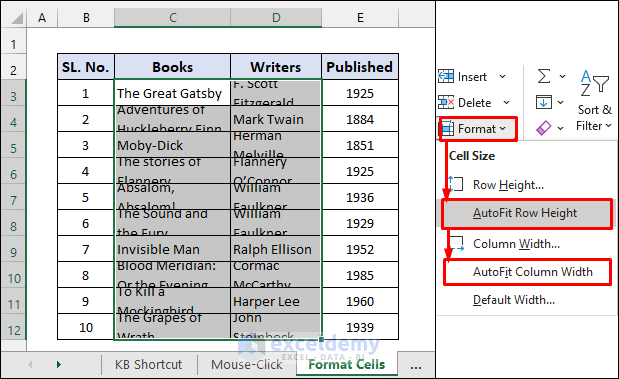
Alternatively, you can get the same result using cell formatting. Just select the cells containing the wrap texts. Then select Format >> AutoFit Row Height or AutoFit Column Width from the Home tab.

Read More: How to Wrap Text in Excel Cell

4. Add Magic Buttons from the Quick Access Toolbar to Auto Fit Row Height of Wrap Text

If you need to do this often, then you should probably add a magic button in the Quick Access Toolbar.

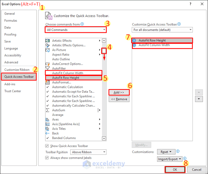
• First, press ALT+F+T to open Excel Options. Then select the Quick Access Toolbar tab. Next, choose All Commands from the dropdown list. After that, scroll down to find the AutoFit Row Height or the  AutoFit Column Height command. Then select it and then click the Add button. After that, hit the OK button.

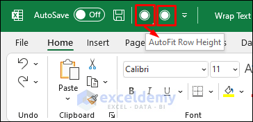
• Now you will see a magic button added at the top left corner of the Excel window as a Quick Access Tool. You can use this button to auto-fit the row height of wrap texts in just one click.

Things to Remember

• AutoFit Row Height and AutoFit Column Width features in Excel do not work with merged cells. You need to manually adjust the row height or column width in that case. Excel shows this behavior by design.
• If you apply autofit row height in a range of cells beforehand then the row height will adjust automatically whenever wrap text is applied in those cells.

Download Practice Workbook

You can download the practice workbook from the download button below.

Conclusion

Now you know 4 different methods on how to auto-fit row height or column width of wrap text in Excel. Please let us know which method you prefer the most. You can also use the comment section below for further queries or suggestions. Stay with us and keep learning.

Related Articles

• How to Wrap Text in Merged Cells in Excel
• How to Wrap Text across Multiple Cells without Merging in Excel
• How to Write a Paragraph in Excel Cell
• [Solution:] Excel Wrap Text Not Working for Merged Cell
• Excel VBA to Wrap Text
• VBA to Wrap Text for Entire Sheet in Excel
• How to Use Excel VBA to Unwrap Text

<< Go Back to Wrap Text | Text Formatting | Learn Excel