How to Autofit Row Height with Wrap Text Using Excel VBA (5 Methods)

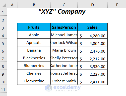
Scenario

In this guide, we’ll address the issue of salesperson names not fitting within cells in an Excel dataset. By using VBA (Visual Basic for Applications) code, we’ll dynamically adjust row heights and wrap text to ensure clear visibility.

Note: We’re using Microsoft Excel 365 in this example, but you can adapt these methods to other Excel versions as needed.

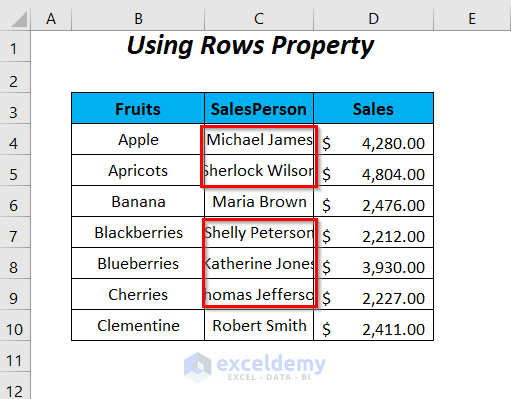
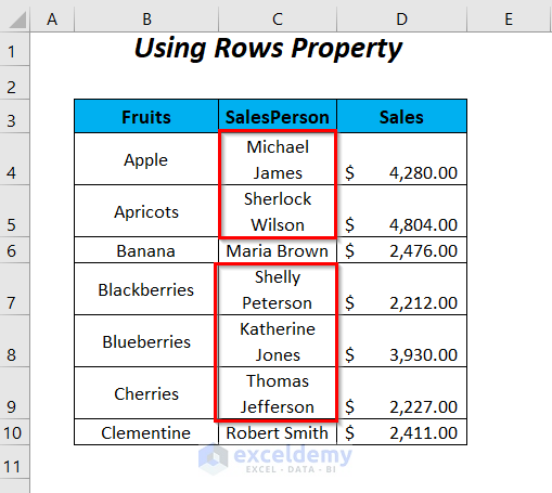
Method 1 – Autofit Row Height Using VBA Rows Property

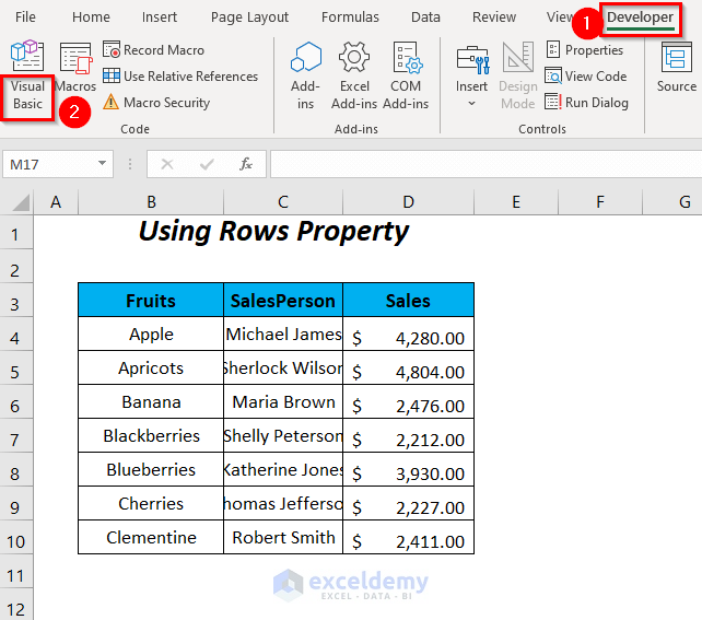
• Open the Visual Basic Editor:
  • Go to the Developer tab and click on Visual Basic.

• • The Visual Basic Editor window will open.

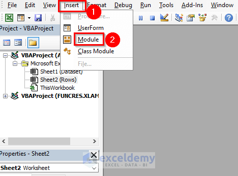
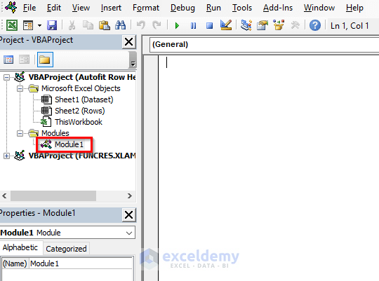
• Create a Module:
  • In the Visual Basic Editor, go to the Insert tab and select Module.

• • Enter the following code

Sub automation_of_row_height_with_text_1()

Rows("4:10").WrapText = True
Rows("4:10").EntireRow.AutoFit

End Sub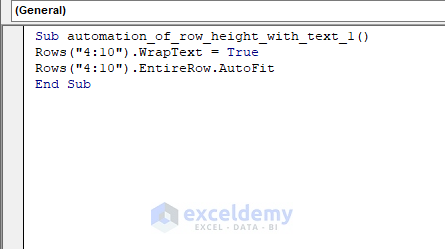

• • Press F5 to execute the code.
  • This will adjust row heights for the salesperson names in cells C4 to C10.

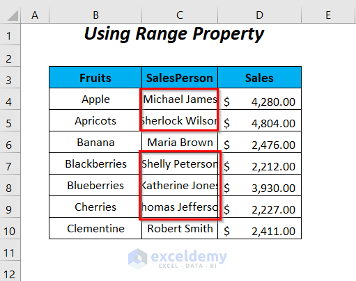
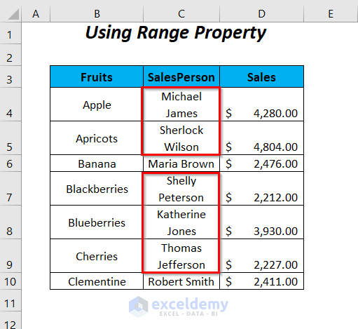
Method 2 – Autofit Row Height Using VBA Range Property

• Create Another Module:
  • Follow the same steps as in Method 1 to create a new module.
• Enter the Code:
  • Enter the following code:

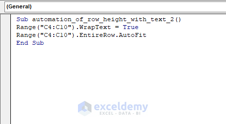
Sub automation_of_row_height_with_text_2()

Range("C4:C10").WrapText = True
Range("C4:C10").EntireRow.AutoFit

End Sub

• This code wraps the text in cells C4 to C10 and adjusts row heights accordingly.

• Execute the Code:
  • Press F5 to run the code.
  • Now the salesperson names will be properly fitted and visible in the SalesPerson column.

Remember to adapt the cell ranges and adjust the code as needed for your specific dataset. These methods ensure that text is wrapped and row heights are adjusted dynamically.

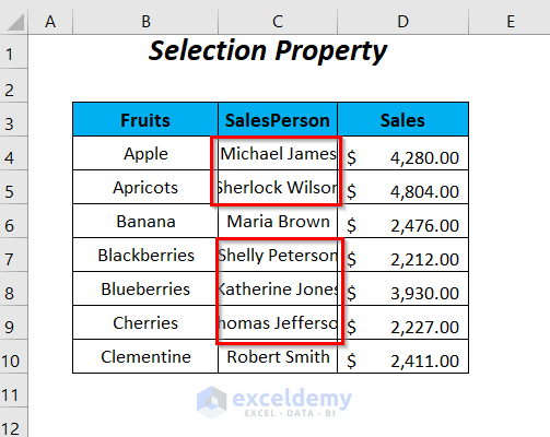
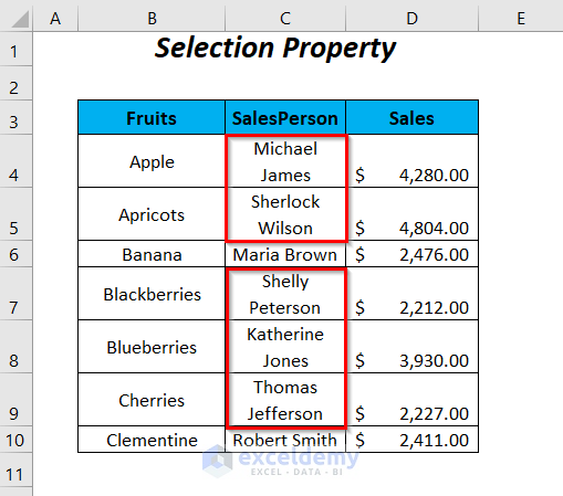
Method 3 – Using Selection Property to Autofit Row Height with Wrap Text

To make the salesperson names visible, we’ll wrap the text and automatically adjust row heights in the SalesPerson column using the Selection property.

Steps:

• Open the Visual Basic Editor:
  • Go to the Developer tab and click on Visual Basic.
  • The Visual Basic Editor window will open.
• Enter the Code:
  • Enter the following code:

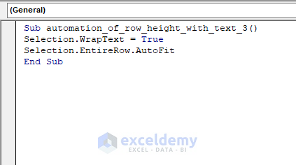
Sub automation_of_row_height_with_text_3()

Selection.WrapText = True
Selection.EntireRow.AutoFit

End Sub

The Selection property considers the range you select. With WrapText = True, it wraps the text, and EntireRow.AutoFit adjusts row heights for clear visibility.

• Execute the Code:
  • Save the code and return to the main sheet.
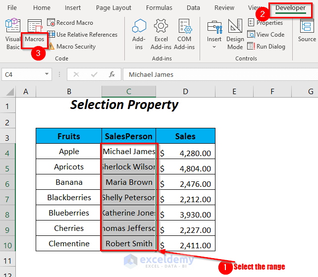
  • Select the desired range.
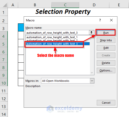
  • Go to the Developer tab >> Macros option.

• • In the Macro dialog box, choose the macro name AutofitRowHeight3 and press Run.

• You’ll see the Salesperson names wrapped and row heights adjusted to accommodate them properly.

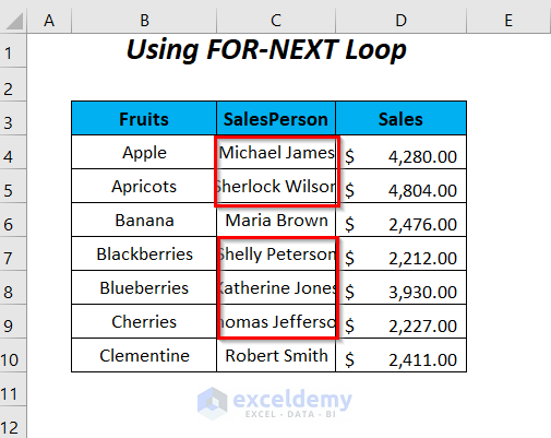
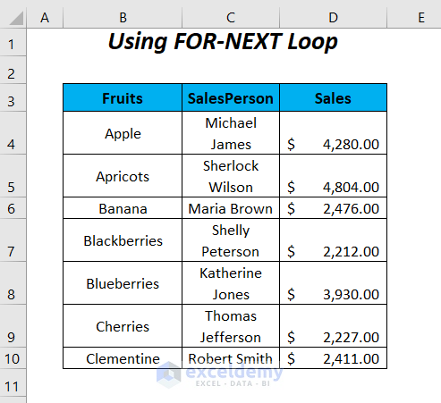
Method 4 – Using FOR-NEXT Loop to Autofit Row Height and Wrap Text

Steps:

• Follow Step 1 of Method-1.

• Enter the Code:
  • Enter the following code:

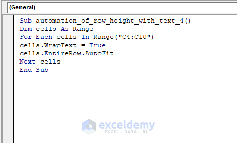
Sub automation_of_row_height_with_text_4()

Dim cells As Range

For Each cells In Range("C4:C10")
cells.WrapText = True
cells.EntireRow.AutoFit
Next cells

End Sub

• • • This loop iterates through each cell in the range C4:C10, wrapping text and adjusting row heights.

• Execute the Code:
  • Press F5 to run the code.
  • Now the names will be visible after autofitting rows with wrapped text in the SalesPerson column.

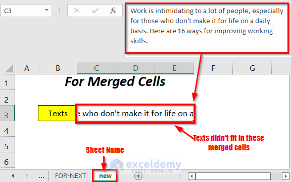
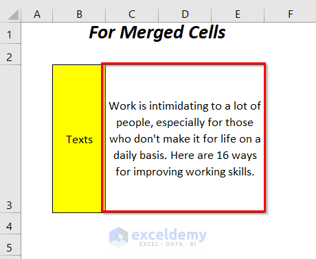
Method 5 – Autofit Row Height Wrap Text for Merged Cells

• Follow Step-01 of Method-1.
• Enter the Code:
  • Enter the following code:

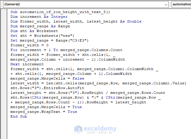
Sub automation_of_row_height_with_text_5()

Dim increment As Integer
Dim former_width, latest_width, latest_height As Double
Dim merged_range As Range
Dim sht As Worksheet
Set sht = Worksheets("new")
Set merged_range = Range("C3:E3")

former_width = 0
For increment = 1 To merged_range.Columns.Count
former_width = former_width + sht.cells(1, _
merged_range.Column + increment - 1).ColumnWidth
Next increment
former_width = sht.cells(1, merged_range.Column).ColumnWidth _
+ sht.cells(1, merged_range.Column + 1).ColumnWidth
merged_range.MergeCells = False
latest_width = Len(sht.cells(merged_range.Row, merged_range.Column).Value)
sht.Rows("3").EntireRow.AutoFit
latest_height = sht.Rows("3").RowHeight / merged_range.Rows.Count
sht.Rows(CStr(merged_range.Row) & ":" & CStr(merged_range.Row _
+ merged_range.Rows.Count - 1)).RowHeight = latest_height
merged_range.MergeCells = True
merged_range.WrapText = True

End Sub

• • • This code adjusts row heights and wraps text for merged cells in the range C3:E3.

• Execute the Code:
  • Press F5 to run the code.
  • The text strings will be visible after wrapping and increasing row heights for merged cells.

Practice Section

A practice section has been provided, as shown below in a sheet named Practice.

Download Practice Workbook

You can download the practice workbook from here: