How to Wrap Text Automatically in Excel – 5 Methods

This is an overview:

Method 1 – Wrap Text in Excel by Format Cells Option

Steps

• Select the cell that contains text that needs to be wrapped.

• Right-click and select Format Cells.

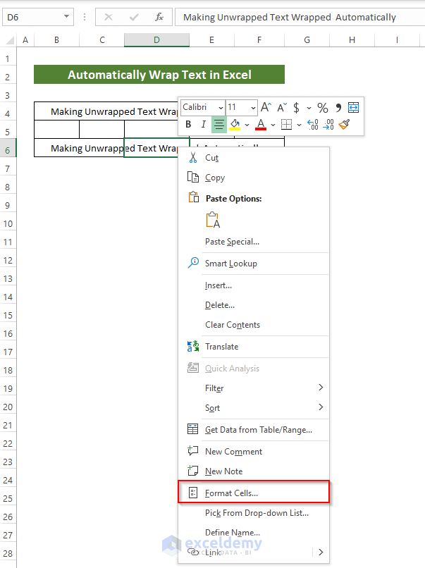
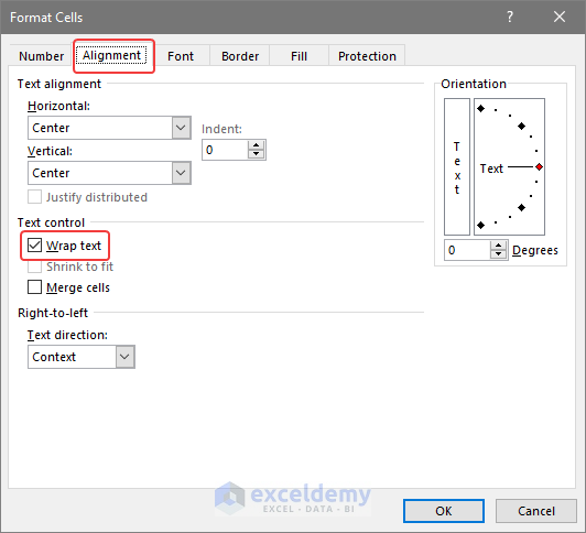
• Select Text control in Alignment.
• Check Wrap Text.
• Click OK.

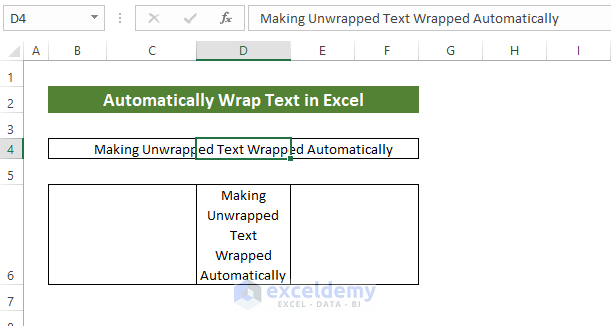
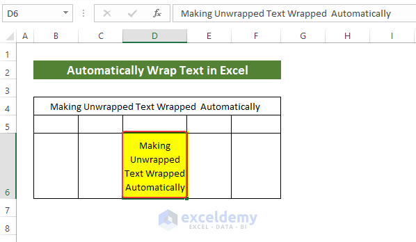
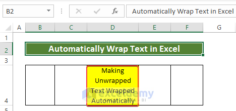
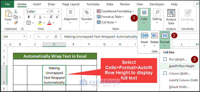
Text in D6 is wrapped.

You can change the Row height to see all the text.

Method 2 – Wrap Text in Excel Using the Ribbon

Steps

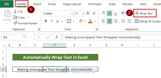
• Select the cell that contains text that needs to be wrapped.
• Go to the Home tab and click Wrap Text in Alignment.

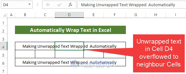
• Text in D4 is wrapped.

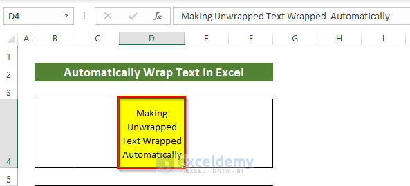
Adjust the Row height to see all the text.

Read More: How to Wrap Text in Excel Cell

Method 3 – Wrap Text Using a Shortcut

Steps

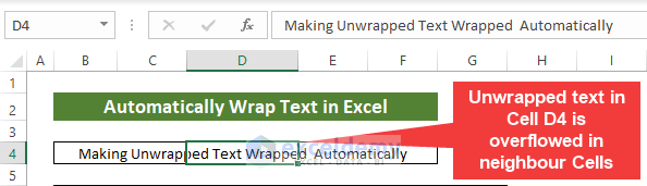
• The text in D4 is too long to fit into one cell.

• Select D4 and press Alt > H > W one by one.

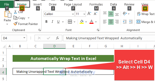
• The text is wrapped.

Adjust the row height to see all the text.

Read More: Wrap Text in Excel Shortcut Key

Method 4 – Insert Manual Line Breaks to Wrap Text in Excel

Steps

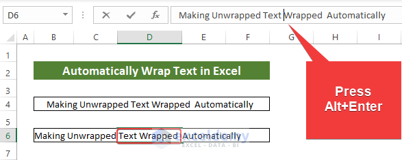
• Select the cell that contains the text that needs to be wrapped. Here, D6.
• Double-click the cell to enable edit mode or press F2.
• Place the cursor where you want to break the text.
• Press Alt+Enter.

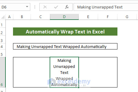
It will break the line into two parts.

• Insert more line breaks if necessary.

Method 5 – Using VBA to Wrap Text Automatically

Use a VBA Macro to wrap text in Excel.

Steps

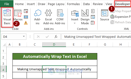
• Go to the Developer tab and click Visual Basic.

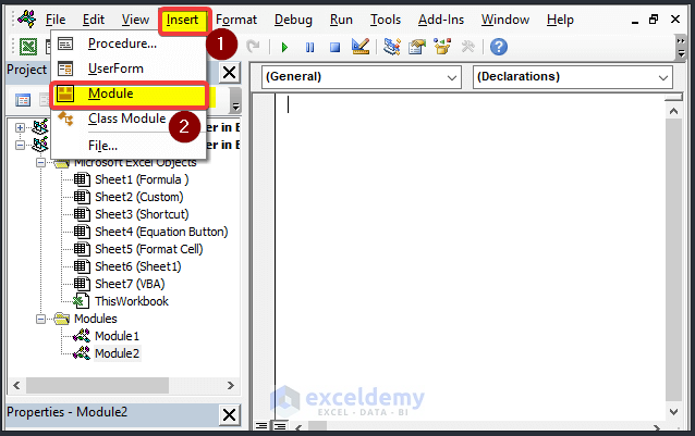
• Click Insert and choose Module.

• Enter the following code:

Sub wrap_text()

  Range("D4").WrapText = True

End Sub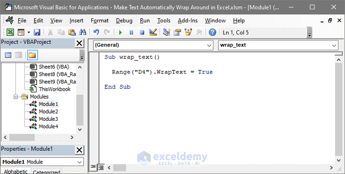

• Close the window.
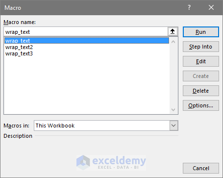
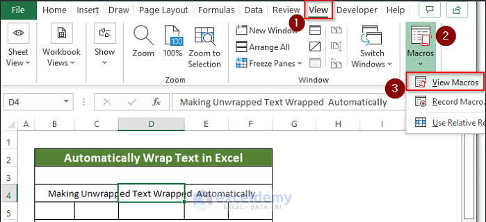
• Go to the View tab > Macros > View Macros.

• Select the macro you created (here, wrap_text).
• Click Run.

• The text in D4 is wrapped.

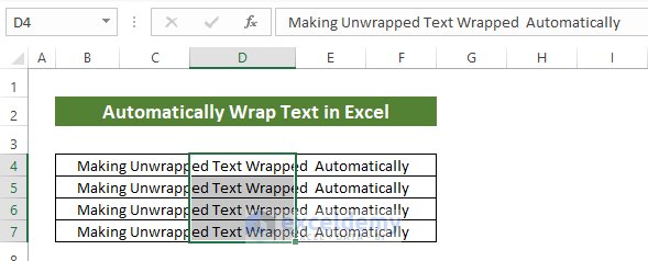
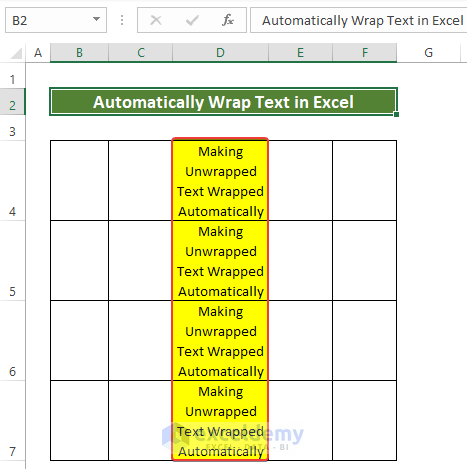
To wrap a range of cells, like in the dataset shown below:

• Enter the following code in the VBA editor:

Sub wrap_text2()

  Range("D4:D7").WrapText = True

End Sub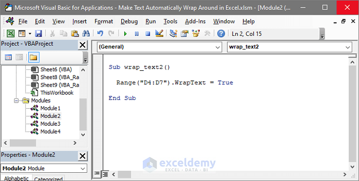

• Close the VBA editor window.
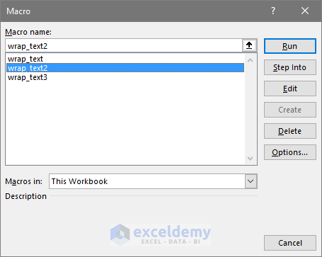
• Go to View tab > Macros > View Macros.

• Select the macro that you created (here, wrap_text2).
• Click Run.

This is the output.

To wrap a whole worksheet, use the following code:

Sub wrap_text3()
ActiveSheet.UsedRange.WrapText = True
End Sub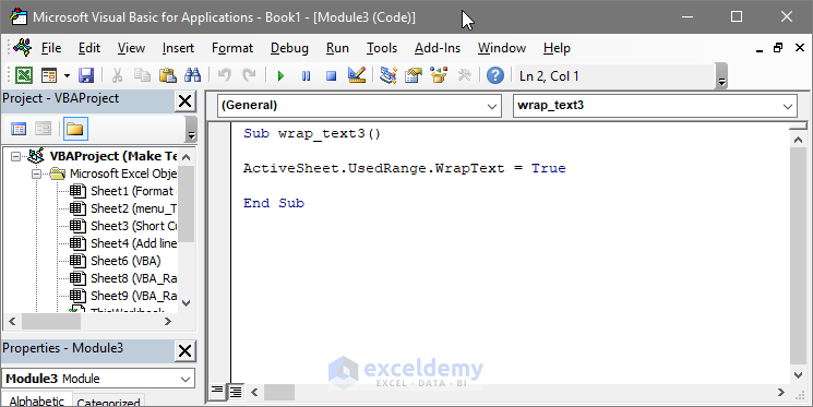

• Close the window.
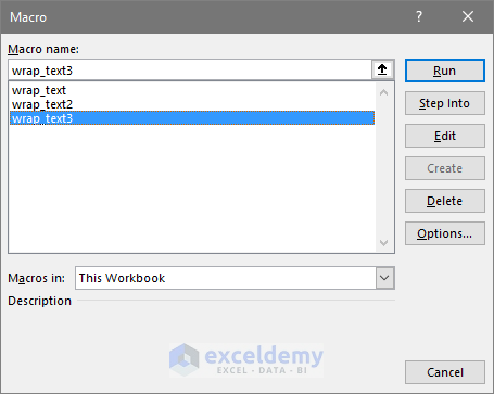
• Go to the View tab > Macros > View Macros.

• Select the macro you created (here, wrap_text3).
• Click Run.

• The text in the whole worksheet is wrapped.

Download Practice Workbook

Download the practice workbook.

Related Articles

• [Fix] Wrap Text Not Working in Excel: 4 Possible Solutions
• [Fixed] Wrap Text Not Showing All Text in Excel
• [Fix]: Excel Wrap Text Cutting off Words
• How to Unwrap Text in Excel

<< Go Back to Wrap Text | Text Formatting | Learn Excel