There are lots of functions in Excel to perform specific tasks. One of them is this ODD function. We use this function to get odd values. In this article, we will discuss this Excel ODD function and examples with proper explanations.
Introduction to ODD Function in Excel
The ODD function always returns an odd number. In the case of positive even numbers, it gives the next odd integer. On the other hand, for negative even numbers, it returns the previous odd number.

Syntax:
=ODD(number)
Arguments:
| ARGUMENT | REQUIRED/OPTIONAL | EXPLANATION |
|---|---|---|
| number | REQUIRED | It is the number for which we want the nearest odd integer. |
Return:
In return, we will always get an odd integer.
Available in:
Microsoft Excel 365, Microsoft Excel 365 for Mac, Excel for the Web, Excel 2021, Excel 2021 for Mac, Excel 2019, Excel 2019 for Mac, Excel 2016, Excel 2016 for Mac, Excel 2013, Excel 2010, Excel 2007, Excel for Mac 2011, Excel Starter 2010.
4 Suitable Examples of Using ODD Function in Excel
In this section, we will discuss some examples to help understand the use of the ODD function. For details, have a look at the below examples.
Example 1: Use of ODD Function with Integers
In this example, we will see how the ODD function behaves with positive and negative integer numbers.
1.1 ODD Function with Positive Integers
Look at the following dataset that contains some positive numbers, odd and even.

- Now, apply the following formula to Cell C5.
=ODD(B5)
- Extend this formula to the last cell.
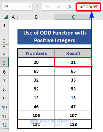
We can see all the numbers in the Result column are converted to odd numbers.
- Again, look at the dataset.

Cell B6 consists of an odd number, and the ODD function does not make any change in the output on Cell C6. It means the ODD function does not have any effect on odd numbers.
But, numbers like 20, 32, 52, etc. in column B are converted to the next odd integer numbers (like, 21, 33, 53, etc.) after applying the ODD function to them.
1.2. ODD Function with Negative Integers
In this example, we will use negative integers as the input values. Then we will observe the effect of applying the ODD function to them.
- Apply the following formula to Cell C5 and extend this to Cell C12.
=ODD(B5)
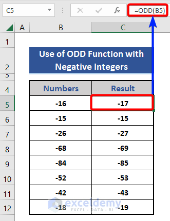
Look at the output the ODD function produces here. It changes nothing of the odd negative numbers. But it converts the negative even numbers.
But unlike the previous example, it now gives you the preceding negative odd numbers,
Example 2: Utilize ODD Function with Fraction Numbers
In the first examples, we have seen the use of the ODD function with integer numbers only. Now let’s see what it does with fractions.
Faction values contain at least one decimal point. But in the return, the decimal section will remove and get odd integers only.
2.1 Positive Fraction Numbers
Say, you have a number, 21.1. It’s a fraction of course. It has one digit after the decimal point. Now, if you apply the ODD function to it, what will happen?
Look at the dataset. We have gathered several fractional numbers here. And all of them are positive numbers.

- Put the following formula on Cell C5.
- Expand this formula till Cell C12 using the Fill Handle feature.
=ODD(B5)
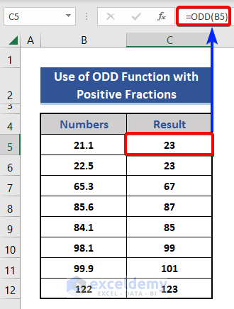
So, the ODD function, in this case, is giving us the next odd integer number skipping the even integer number in between.
2.2 Negative Fraction Numbers
What happens to negative fractions? Let’s see this using some random fraction like the image below.

- Apply the formula on Cell C5.
=ODD(B5)
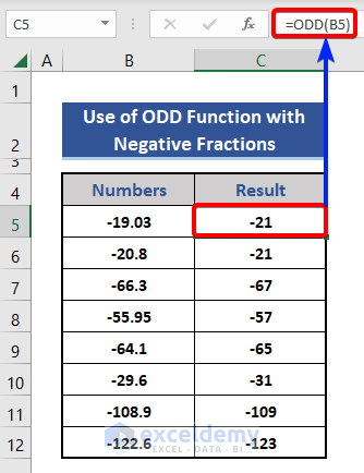
Since the numbers are negative, the ODD function goes back and picks the preceding negative integer numbers.
For example, it returns -21 for -19.03. Because the last negative number before -19 is -21.
Example 3: Use ODD Function in Excel VBA
The ODD function is also available in Excel VBA. Let’s see another example to clarify how to use it in case of VBA.
- First, we inserted some numbers in the dataset.
- Then, go to the Sheet Name section at the bottom of the sheet.
- Press the right button of the mouse.
- Choose the View Code option from the menu.

- The VBA Applications window appears.
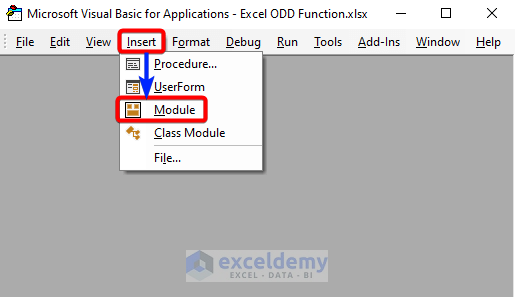
- Choose the Module option from the Insert tab.
- Now, insert the following VBA code on this window.
Sub odd_function()
Dim Input_number, Output_Number As Double
Set Input_number = Application.InputBox("Select Cell", "Cell", Type:=8)
Output_Number = Application.WorksheetFunction.Odd(Input_number)
MsgBox (Output_Number)
End Sub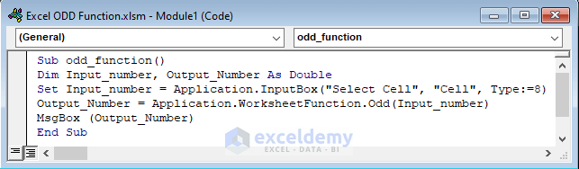
- Run the code by pressing the F5 button.
- A dialog box will appear to choose cells from the dataset.
- Select any cell and press the OK button.

- Finally, a message box appears.

So, we can see that the VBA Odd function works exactly the same way as the Excel ODD function.
Example 4: Find and Count Odd Numbers with ODD function
Here, we will mark the odd (or even numbers) and count them using the IF and COUNTIF functions in Excel.
- We have a list of numbers. Some of them are odd, some even, and the rest are not any of them will be marked as N/A.

- Apply the following formula on Cell C5 based on the nested IF function.
- Drag the formula till Cell C12.
=IF($B5=ODD($B5),"Odd",(IF($B5=EVEN($B5),"Even","N/A")))
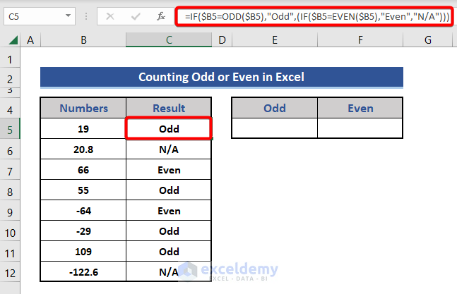
We can see the numbers have been marked.
- Now, use formulas based on the COUNTIF function on Cells E5 and F5.
For Cell E5:
=COUNTIF($C$5:$C$12,E4)
For Cell F5:
=COUNTIF($C$5:$C$12,F4)
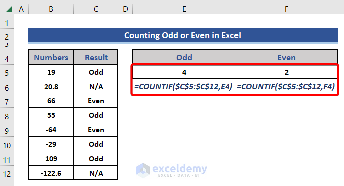
We get the total number of odd and even numbers separately.
Things to Remember
- For any non-numeric value, the ODD function will return #VALUE!
- The ODD function has no effect on even numbers.
Download Practice Workbook
Download this practice workbook to exercise while you are reading this article.
Conclusion
I hope, after reading this article, it’s clear to you how the ODD function works and how to use it in different cases. If you have any further queries, please let me know in the comment box. I will try to reply as soon as possible.
<< Go Back to Excel Functions | Learn Excel
Get FREE Advanced Excel Exercises with Solutions!

Thank you very much for all this examples . Please ,
can you show how to delete odd or even numbers in a range with a VBA code ?
Thanks Nicu for reaching us out. To delete odd or even numbers in a range, you can use the following VBA Code:
After running the code, an InputBox will ask you to select a range from where you want to delete numbers. Then, another InputBox will appear asking you to input 0 for deleting even numbers and 1 for deleting odd numbers. After inserting the number, the cells containing even/odd numbers will be deleted based on your input. I hope the code solves your problem. If you have any further queries, feel free to comment.
Regards
Aniruddah
Team Exceldemy