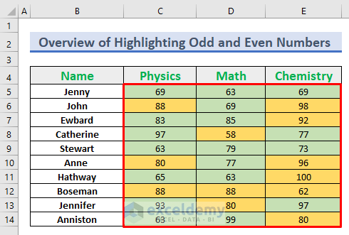
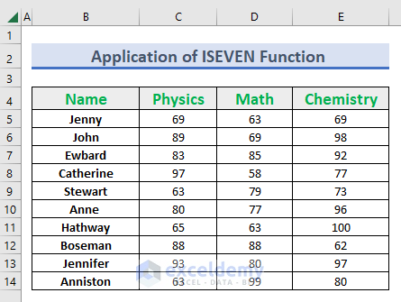
While working with large data sets in Microsoft Excel, you may need to highlight odd and even numbers from the worksheet because of the convenience of our work. This article will cover the easiest ways of highlighting even and odd numbers using conditional formatting in Excel. After reading this article you will be able to highlight even and odd numbers in Excel files. Here is the overview of today’s dataset.
How to Apply Conditional Formatting in Excel to Highlight Odd and Even Numbers: 3 Examples
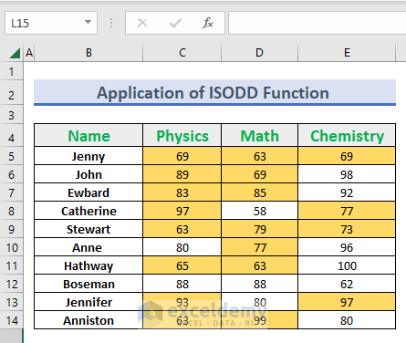
To highlight even and odd numbers, there are ample methods available online. Of them, the three methods below are quite efficient and quick to learn and practice in real-life Excel problem-solving. Let’s say, we have a dataset of several students’ marks in Physics, Chemistry, and Mathematics at XYZ school. We will apply the MOD, ISEVEN, ISODD, and ROW functions to highlight odd and even numbers with conditional formatting. All three methods will be discussed step by step.
1. Highlight Odd and Even Numbers Using MOD Function with Conditional Formatting
In this method, we will apply the MOD function with Conditional Formatting to highlight odd and even numbers in Excel. Let’s follow the instructions below to learn!
i. Highlight Even Numbers
Now, we will highlight even numbers using the MOD function with Conditional Formatting. Let’s follow the steps below to learn!
Steps:
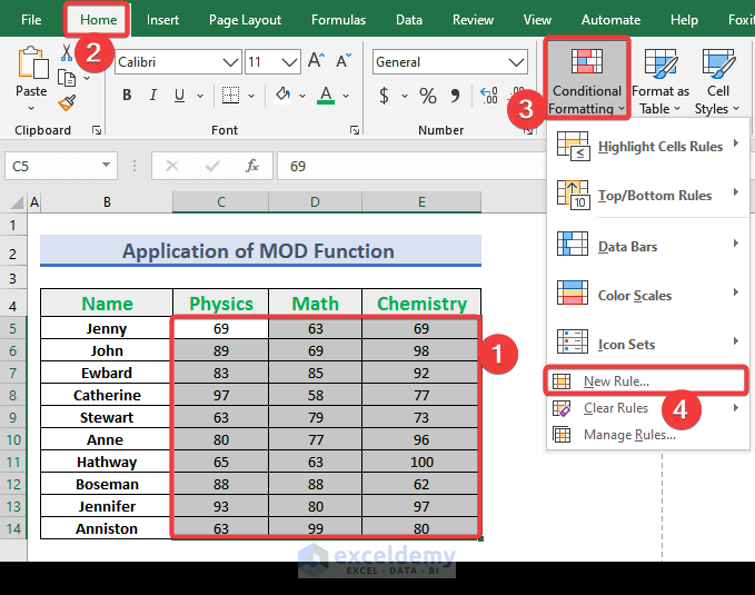
- First, select cells from C5 to E14 to apply the conditional formatting. Then, from your Home tab, go to,
Home → Styles → Conditional Formatting → New Rule
- A dialog box named New Formatting Rule will appear. Follow the steps for the New Formatting Rule dialog box.
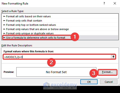
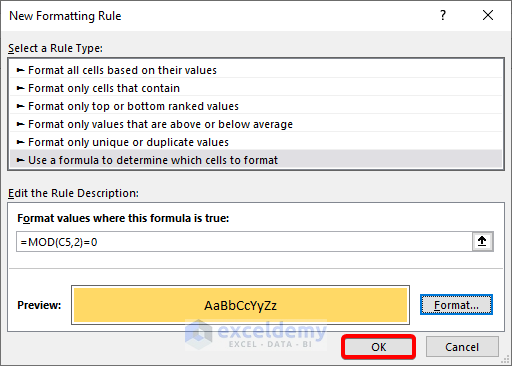
- First, select Use a formula to determine which cells to format from the Select a Rule Type:
- Next, write the below formula in the Format values where this formula is true:
- The MOD function is,
=MOD(C5,2)=0- Hence, press the Format option.
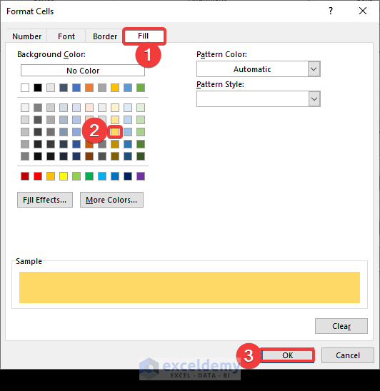
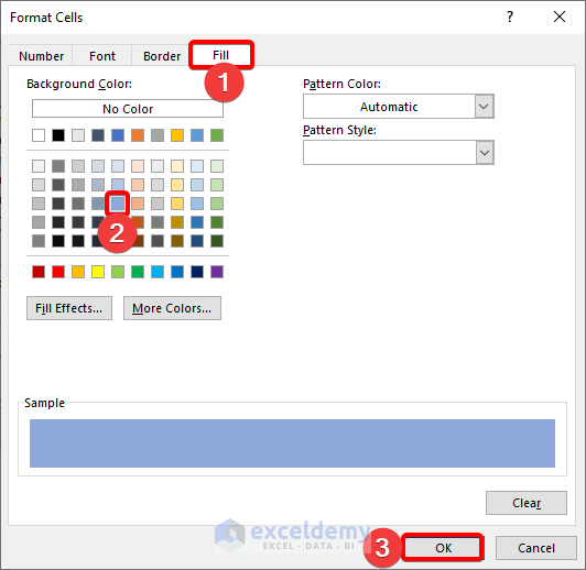
- After clicking on the Format option, a Format Cells dialog box pops up.
- First, select the Fill ribbon from that dialog box
- Next, select any color from the Background Color menu. We have chosen light yellow. At last, click OK.
- After that, again press OK.
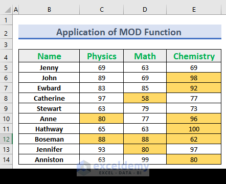
- Finally, the even numbers are highlighted with the desired color in the data table.
ii. Highlight Odd Numbers
The process of highlighting even numbers follows the same process as highlighting odd numbers. So, if you learn the above process, this will be quite easier for you to execute. You just have to change the formula in the New Rule tab.
Steps:
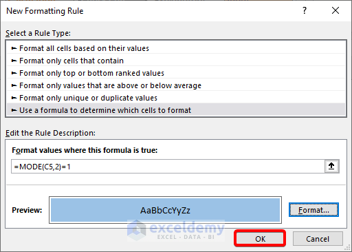
- First, select cells from C5 to E14 to apply the conditional formatting. Hence, open the New Formatting Rule window and insert the below formula in the Format values where this formula is true:
- The formula is,
=MOD(C5,2)=1- Hence, press the Format option.
- After that, you will choose a color from the Fill We have chosen light blue. At last, click OK.
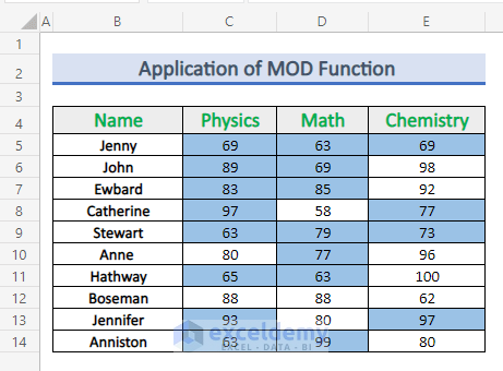
- Finally, the highlighted odd numbers appear as follows.
2. Use ISEVEN or ISODD Rule in Conditional Formatting to Highlight Odd or Even Numbers
In this section, we will apply the ISEVEN and ISODD functions to highlight even or odd numbers with conditional formatting in Excel. Let’s follow the instructions below to learn!
i. Use ISEVEN Function to Highlight Even Number
To understand the method, let’s assume a dataset below. It contains real-life data of students and their obtained marks in different subjects.
Steps:
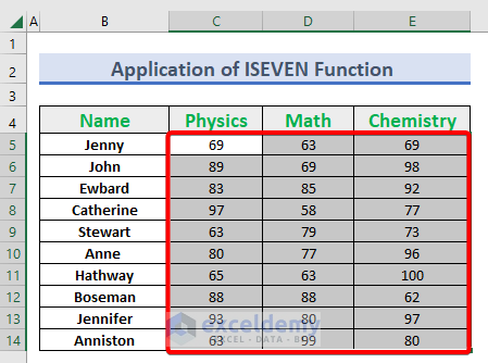
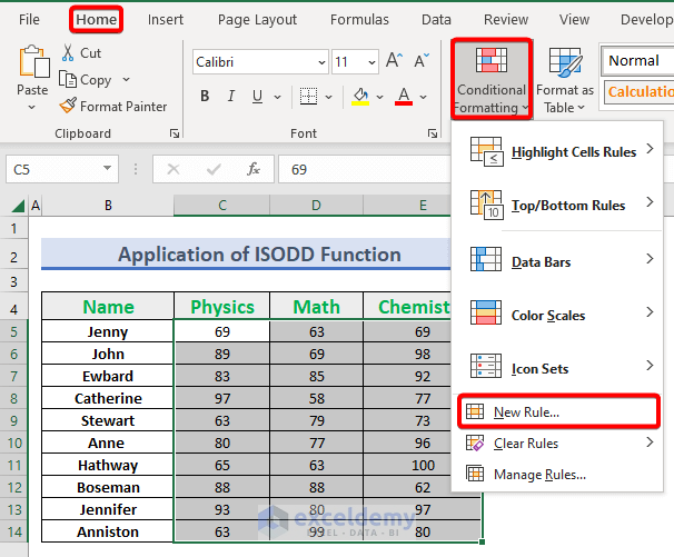
- First, From C5 to E14 cells must be selected to apply the conditional formatting.
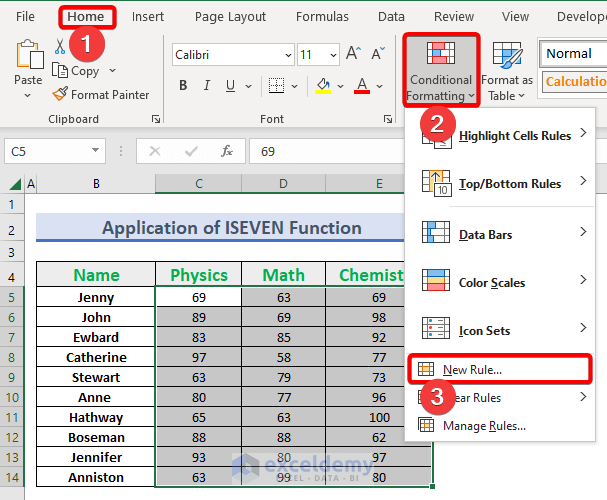
- Then, from your Home tab, go to,
Home → Styles → Conditional Formatting → New Rule
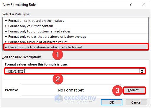
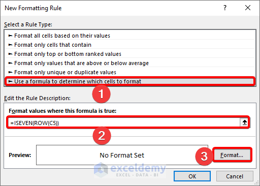
- After clicking New Rule, the New Formatting Rule Tab opens. From there you have to select “Use New Formula to Determine which cells to format” from Select a New Rule Type. There you have to write a formula as
=ISEVEN(C5)- Then you have to click “Format” from the tab.
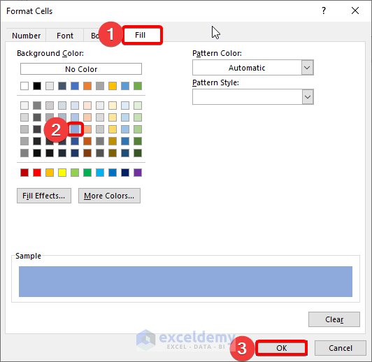
- After clicking Format, the following tabs pop up. You can select the preferred color that you would like to see. The color will be used to visualize the even numbers in the dataset.
- In Format Cell, I have pressed Fill tab. Then, I selected a light violet color and then pressed OK.
- Then, from the following tab press OK to continue for the final step.

- Finally, the even numbers will appear in a highlighted.

ii. Insert ISODD Function to Highlight Odd Number
Here, highlighting odd numbers using the ISODD function will be discussed. It follows the same steps as the previous method of highlighting even numbers. So, before starting this one, please make sure you understand the previous one.
We will be working on the same dataset as the previous one thus you can understand it properly.
Steps:
- As in the previous one, you have to select from C5 to E14 in the dataset.
- Then, from your Home tab, you have to go to,
Home → Styles → Conditional Formatting → New Rule
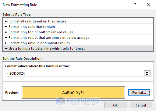
- From the New Formatting Rule, you have to select “Use New Formula to Determine which cells to format” from Select a New Rule Type. There you have to write a formula as
=ISEVEN(C5)- in Format Cell, I have pressed Fill tab. Then, you have to select the light yellow color and then press.
- Then, from the tab press OK.
- Finally, odd numbers are highlighted.
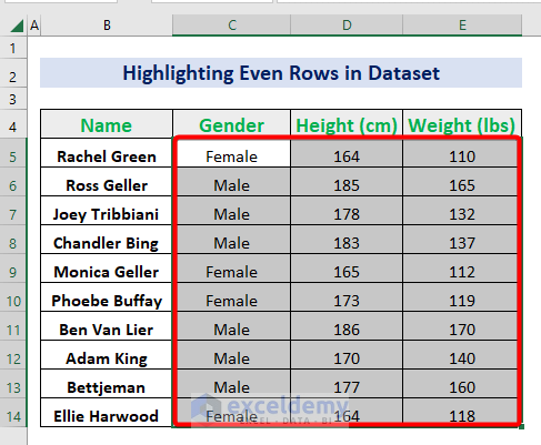
3. Highlight Odd or Even Rows Combining ROW Function with ISEVEN or ISODD
Sometimes, identifying Even and Odd Row distinctively is necessary for a big data set from real life. It helps to differentiate between data of two adjacent rows. To do this, we will be using a combination of both ISODD, ISEVEN, and ROW functions.
i. Highlight Even Rows
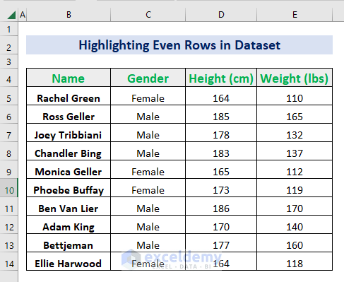
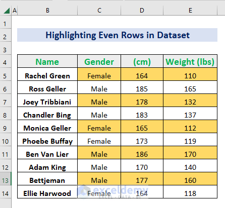
To demonstrate the process, let’s consider a real-life dataset below. It shows people’s names, gender, height, and weight in a consecutive manner.
Steps:
- To begin, select cells from C5 to E14 to apply the conditional formatting.
- Then, from your Home tab, go to,
Home → Styles → Conditional Formatting → New Rule
- A dialog box named New Formatting Rule will appear. Follow the steps for the New Formatting Rule dialog box.
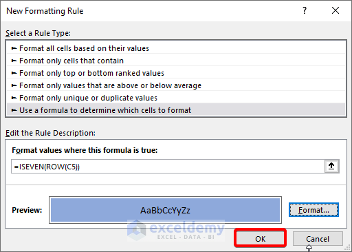
- First, select Use a formula to determine which cells to format from the Select a Rule Type:
- Next, write the below formula in the Format values where this formula is true:.
- The ISEVEN function is,
=ISEVEN(ROW())- Hence, press the Format option.
- After clicking on the Format option, a Format Cells dialog box pops up.
- From that dialog box, first, select the Fill ribbon.
- Next, select any color from the Background Color menu. We have chosen light blue. At last, click OK.
- Hence, you will go back to the New Formatting Rule dialog box. Finally, you have to click OK.
- Finally, you will be able to highlight every even row that has been given in the below screenshot.

ii. Highlight Odd Rows
To highlight odd rows using ISODD and ROW functions, we will be using the same dataset. The process is quite similar to the previous one of highlighting even rows.
Steps:
- First of all, select cells from C5 to E14 to apply the conditional formatting. Then, from your Home tab, go to,
Home → Styles → Conditional Formatting → New Rule

- A dialog box named New Formatting Rule will appear. Follow the steps for the New Formatting Rule dialog box.
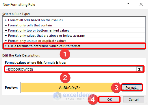
- First, select Use a formula to determine which cells to format from the Select a Rule Type:
- Next, write the below formula in the Format values where this formula is true:
- The ISODD function is,
=ISODD(ROW(C5))- Hence, press the Format option.
- After clicking on the Format option, a Format Cells dialog box pops up.
- From that dialog box, first, select the Fill ribbon.
- Next, select any color from the Background Color menu. We have chosen light Yellow. At last, click OK.
- Finally, you will be able to highlight every odd row that has been given in the below screenshot.
Download Practice Workbook
Download this practice workbook to exercise while you are reading this article.
Conclusion
This whole article covered the thorough process of highlighting even and odd numbers as well as the process of highlighting even and odd rows. Additionally, you can practice this Excel problem by downloading from this page. Yet, if you have any queries related to this problem please comment below.
<< Go Back to | Excel for Math | Excel ODD or EVEN | Learn Excel
Get FREE Advanced Excel Exercises with Solutions!
