Here’s an overview of using Conditional Formatting for multiple conditions.
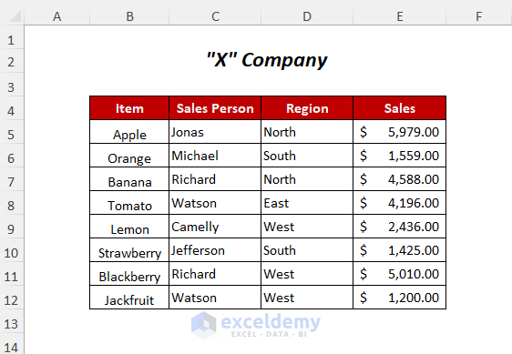
We have the two data tables, which we’ll format. The first table has the sales record for different items of a company
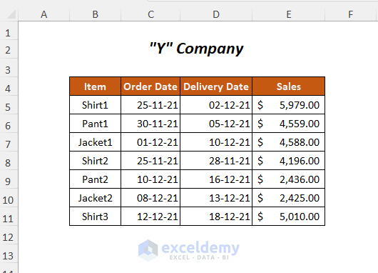
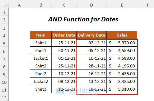
The second table contains the Order Date, Delivery Date, and Sales for some items of another company.
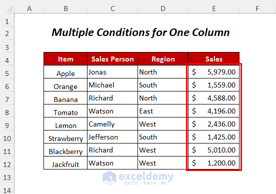
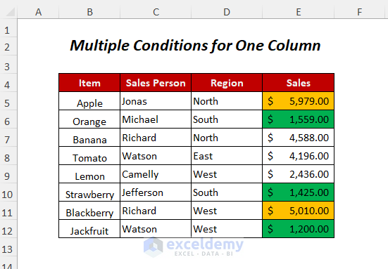
Method 1 – Conditional Formatting for Multiple Conditions in One Column
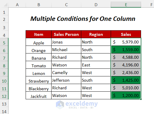
We will highlight the cells of the Sales column containing values less than $2,000.00 and more than $5,000.00.
Steps:
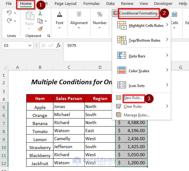
- Select the cell range where you want to apply the Conditional Formatting.
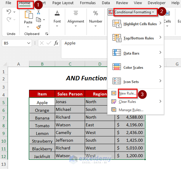
- Go to the Home tab, select the Conditional Formatting dropdown, and choose New Rule.
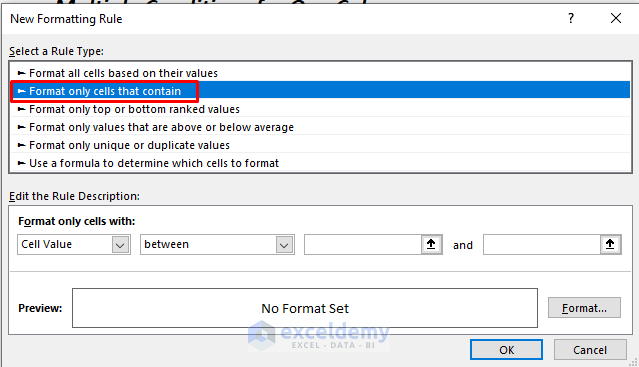
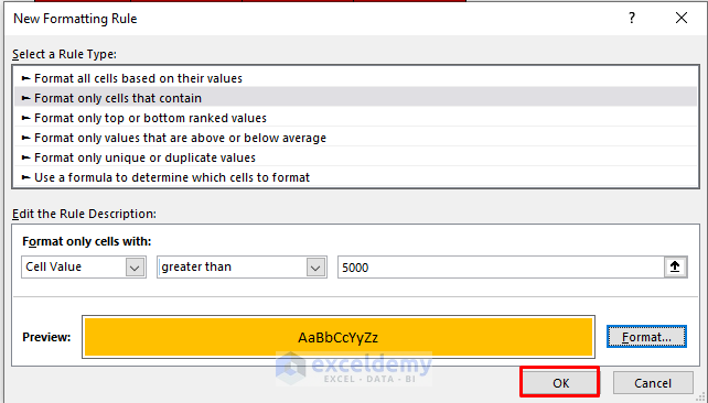
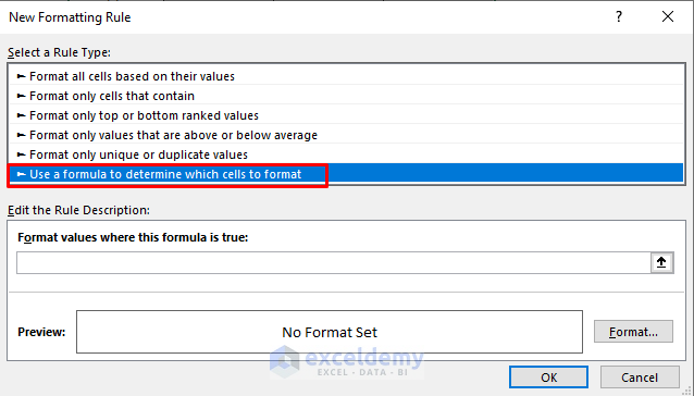
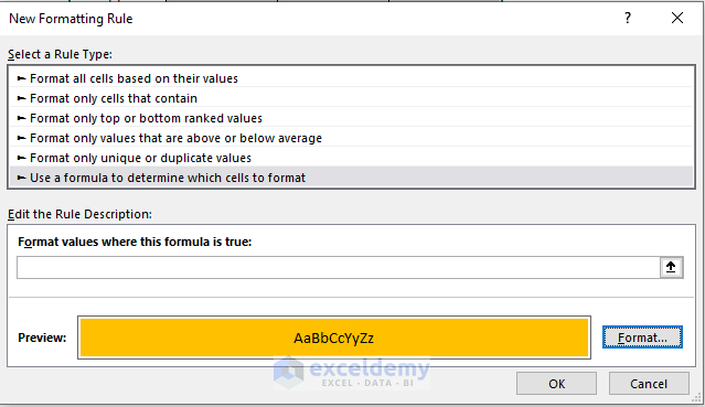
- The New Formatting Rule wizard will appear.
- Select the Format only cells that contain option.
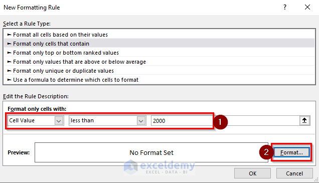
- Choose the following in the Format only cells with: options: Cell Value, less than, 2000.
- Click Format.
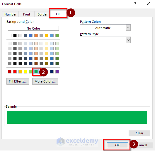
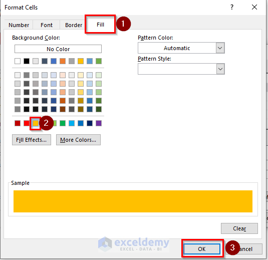
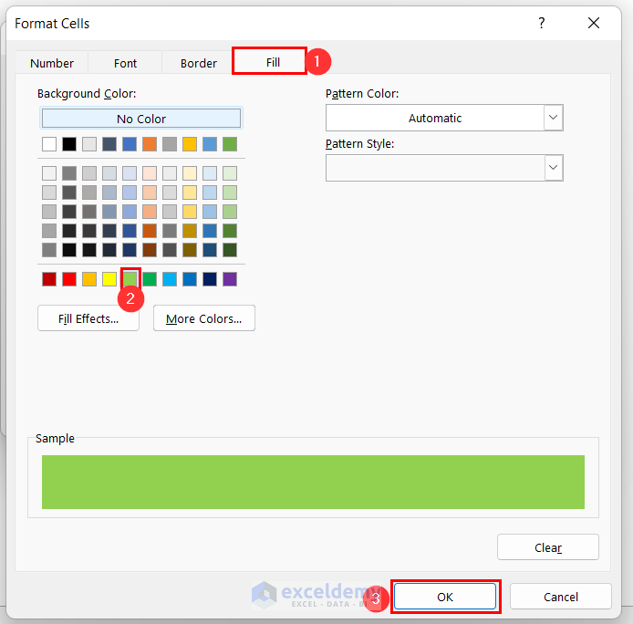
- The Format Cells Dialog Box will open up.
- Select Fill.
- Choose any Background Color.
- Click on OK.
- The Preview will be shown below. Press OK.
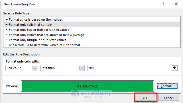
- Press OK again and you will get the cells having a value less than $2,000.00 highlighted.
- Insert a New Formatting Rule for the same range.
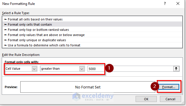
- Choose the following in the Format only cells with settings: Cell Value, greater than, 5000.
- Click Format.
- The Format Cells dialog box will open up.
- Select the Fill option.
- Choose a different Background Color.
- Click on OK.
- The Preview will be shown as below. Press OK.
- Press OK again and you will get the cells highlighted.
Read More: How to Apply Conditional Formatting on Multiple Columns in Excel
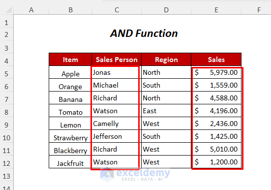
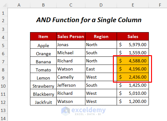
Method 2 – Using the AND Function to Apply Conditional Formatting for Multiple Conditions in Excel
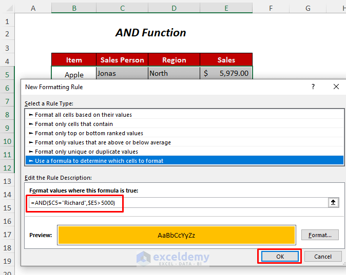
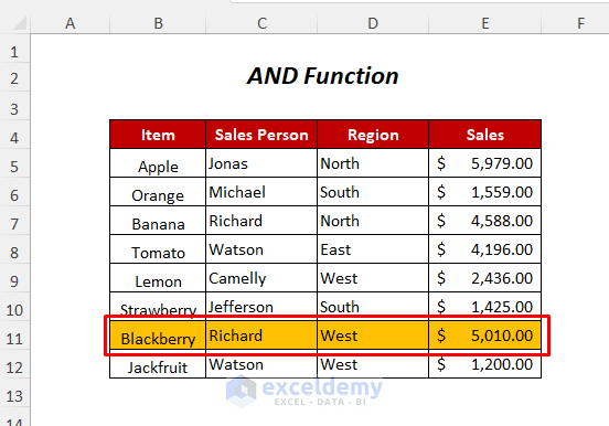
We want to highlight the rows which have a Sales Person named Richard and a sales value greater than $5,000.00.
Steps:
- Select the data range on which you want to apply the Conditional Formatting.
- Go to the Home tab.
- Choose Conditional Formatting.
- Select New Rule.
- The New Formatting Rule wizard will appear.
- Select Use a formula to determine which cells to format.
- Click on Format.

- Choose a color in the Fill tab.
- Click on OK.

- The Preview will be at the bottom.

- Use the following formula in the Format values where this formula is true box:
=AND($C5="Richard",$E5>5000)- Press OK.
- You will get a rows fulfilling both conditions highlighted.
Read More: Conditional Formatting Based on Multiple Values of Another Cell
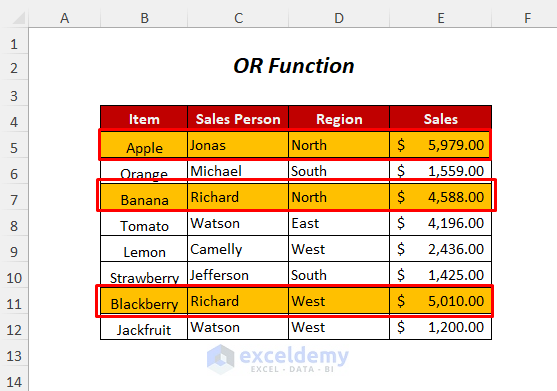
Method 3 – Using the OR Function to Apply Conditional Formatting for Multiple Conditions in One Column
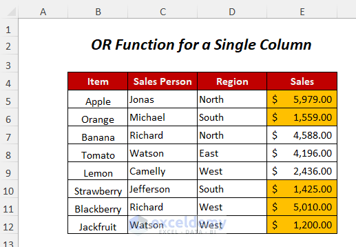
We want to highlight the cells of the Sales column containing values less than $2,000.00 or more than $5,000.00.

Steps:
- Select the column.
- Go to New Rule in Conditional Formatting.

- Use the following formula in the Format values where this formula is true: box.
=OR($E5<2000,$E5>5000)- Choose a color in Format if you want.
- Press OK.
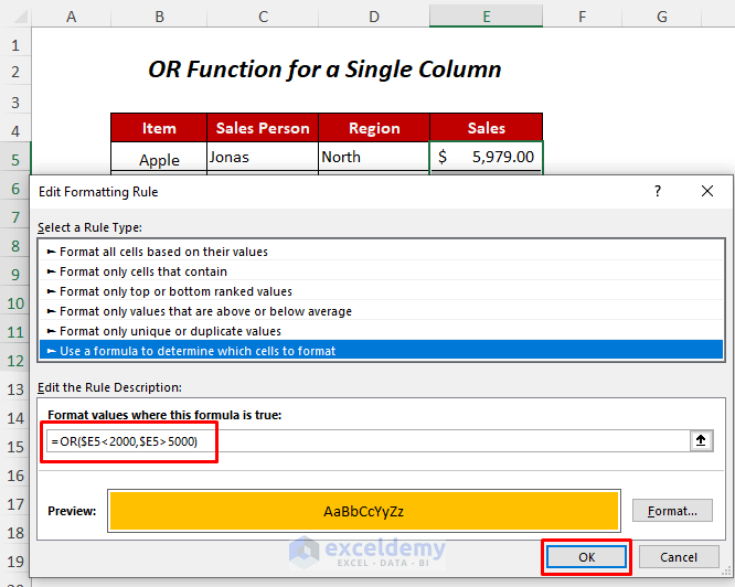
- Here’s the result.
Read More: How to Format Cell Based on Formula in Excel
Method 4 – Conditional Formatting for Multiple Conditions Using the OR Function in Excel
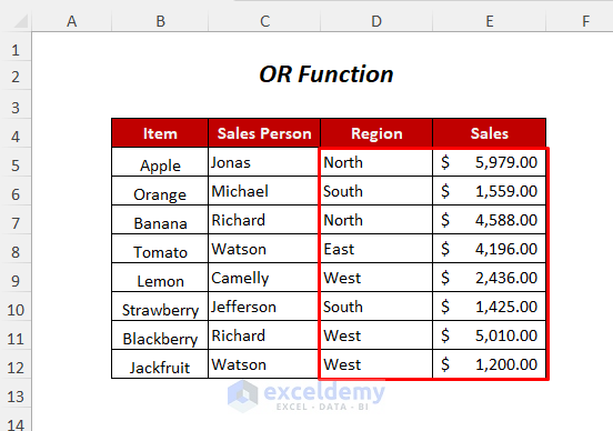
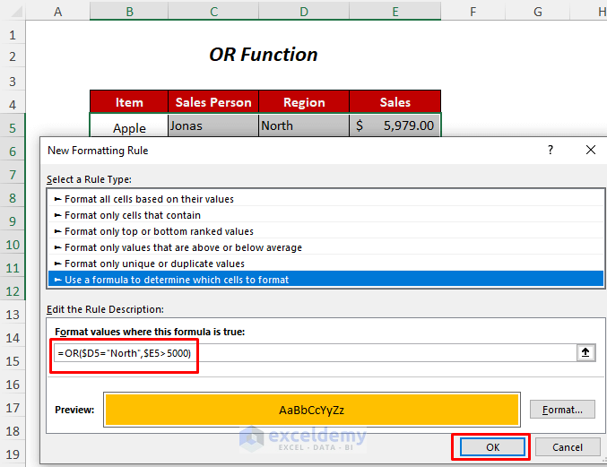
We will highlight the rows in the North Region or which have a sales value greater than $5,000.00.
Steps:
- Select the dataset.
- Go to Conditional Formatting and select New Rule.
- You will get the following New Rule dialog box.

- Use the following formula in the Format values where this formula is true box:
=OR($D5= “North”,$E5>5000)- Press OK.
- Here’s the result.
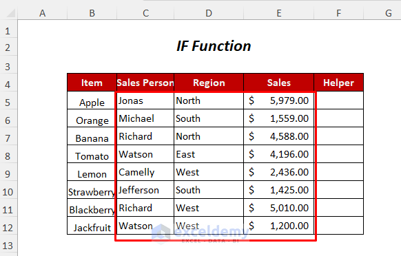
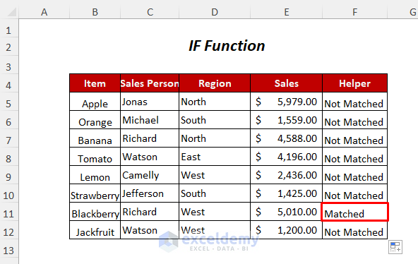
Method 5 – Using the IF Function for Conditional Formatting with Multiple Conditions in Excel
We have added a column named Helper.
Steps:
- Select the output cell F5.
- Insert the following formula:
=IF(C5="Richard",IF(D5="West",IF(E5>5000,"Matched","Not Matched"),"Not Matched"),"Not Matched")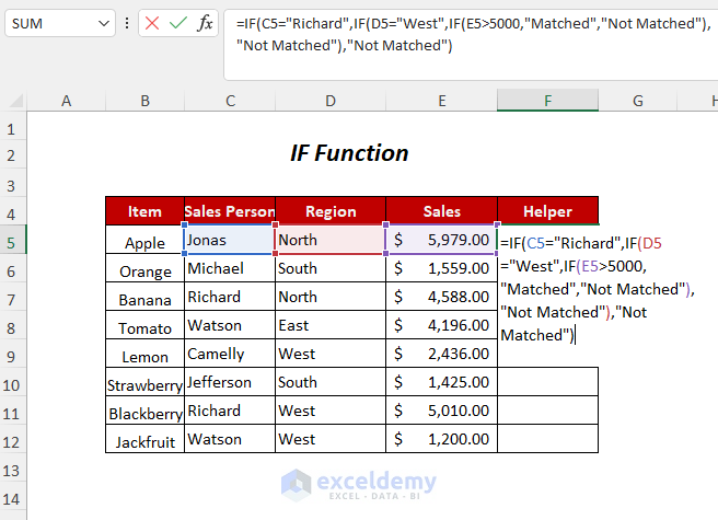
- Press Enter.
- Drag down the Fill Handle tool.
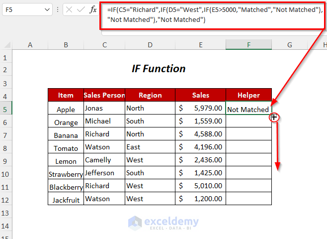
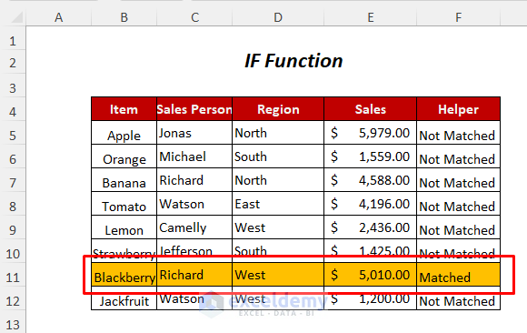
- We will get Matched only for a row where all of the three conditions have been met, and then we will highlight this row.
- Select the cell range where you want to apply the Conditional Formatting.
- Go to the Home tab, select the Conditional Formatting dropdown, and choose New Rule.

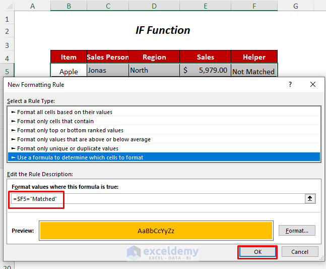
- Use the following formula in the Format values where this formula is true box:
=$F5="Matched"- Press OK.
- Here’s the result.
Read More: Excel Conditional Formatting Formula with IF
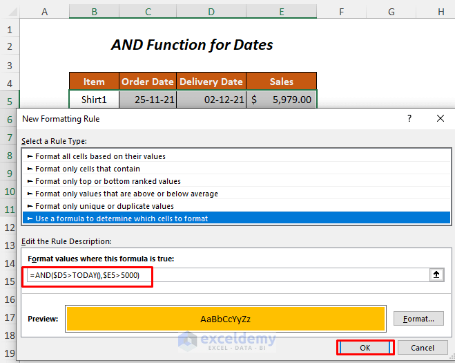
Method 6 – Using the AND Function for Multiple Conditions Including Dates
We want to highlight the rows that have delivery dates after today (today’s date is 12-15-21, and the date format is mm-dd-yy) and a sales value greater than $5,000.00.
Steps:
- Select the cell range where you want to apply the Conditional Formatting.
- Go to the Home tab, select the Conditional Formatting dropdown, and choose New Rule.
- You will get the following New Formatting Rule dialog box.
- Use the following formula in the Format values where this formula is true box:
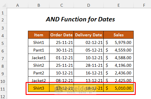
=AND($D5>TODAY(),$E5>5000)- Press OK.
- Here’s the result.
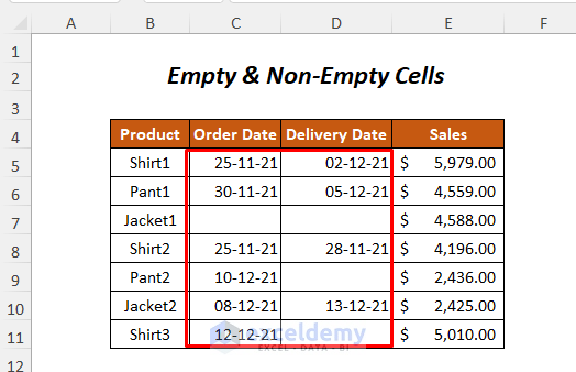
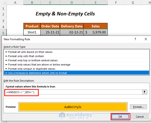
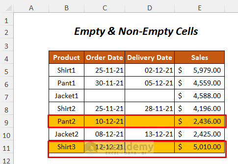
Method 7 – Conditional Formatting for Empty and Non-Empty Cells in Excel
We’ll highlight the sales that have not been delivered (i.e. there’s an order date, but no delivery date).
Steps:
- Select the cell range where you want to apply the Conditional Formatting.
- Go to the Home tab, select the Conditional Formatting dropdown, and choose New Rule.
- You will get the following New Formatting Rule dialog box.

- Use the following formula in the Format values where this formula is true: box:
=AND($C5<>"",$D5="")- Press OK.
- Here’s the result.
Read More: Conditional Formatting for Blank Cells in Excel
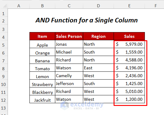
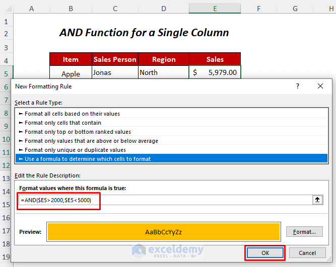
Method 8 – Conditional Formatting for Multiple Conditions in One Column Using the AND Function
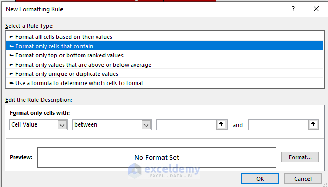
We want to highlight the cells of the Sales column containing values between $2,000.00 and $5,000.00.
Steps:
- Select the cell range where you want to apply the Conditional Formatting.
- Go to the Home tab, select the Conditional Formatting dropdown, and choose New Rule.
- You will get the following New Formatting Rule dialog box.

- Use the following formula in the Format values where this formula is true box:
=AND($E5>2000,$E5<5000)- Press OK.
- Here’s the result.
Download the Practice Workbook
Conditional Formatting for Multiple Conditions in Excel: Knowledge Hub
- Conditional Formatting If Cell is Not Blank
- Change Text Color Based on Value with Excel Formula
- Conditional Formatting Multiple Text Values
- Conditional Formatting Entire Column Based on Another Column
- Excel Highlight Cell If Value Greater Than Another Cell
- VBA Conditional Formatting Based on Another Cell Value
- Change Font Color Based on Value of Another Cell
- Do Conditional Formatting Based on Another Cell
- Conditional Formatting Based on Multiple Values of Another Cell
- Conditional Formatting Based On Another Cell Range
<< Go Back to Conditional Formatting | Learn Excel
Get FREE Advanced Excel Exercises with Solutions!

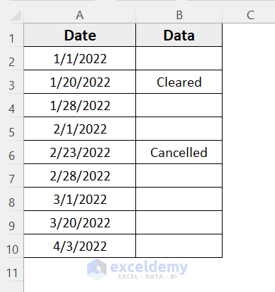
I am trying to do a conditional format when a specific Cell is blank and another cell with a date is less than 30 days, leave blank or greater than 30, 60 or 90 days fill with a color for each category. And if the original cell has a value, ignore the dates and leave blank. As example.
Date Fields are in Column A and Data fields are Column B.
Column A Column B
1/1/2022 Cleared
2/1/2022
3/1/2022 Cancelled
I want to be able to use a multiple value option in Conditional formatting.
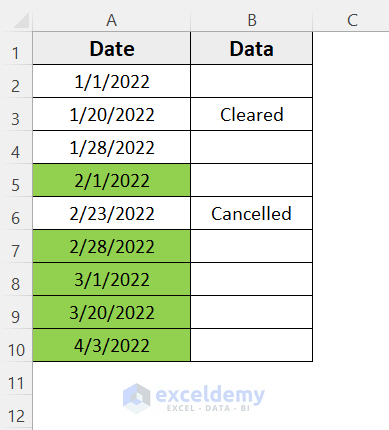
Hello Gabrielle, after going through your problem, I have understood it like this that you want to highlight those dates which are greater than 30 days (or January month) or 60 days (or February month), or 90 days (or March month) and the corresponding specific cells are blank for these dates. If the specific cells are not blank, then the coloring should be avoided. After understanding this scenario, I have created the following dataset like your sample to illustrate the process.
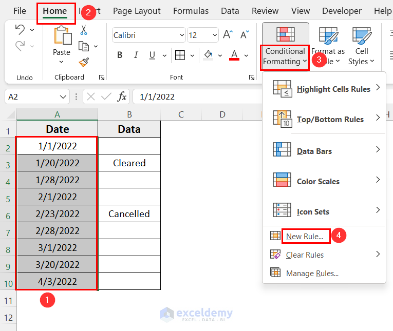
• Firstly, select the dates, and then go to the Home tab >> Conditional Formatting dropdown >> New Rule option.
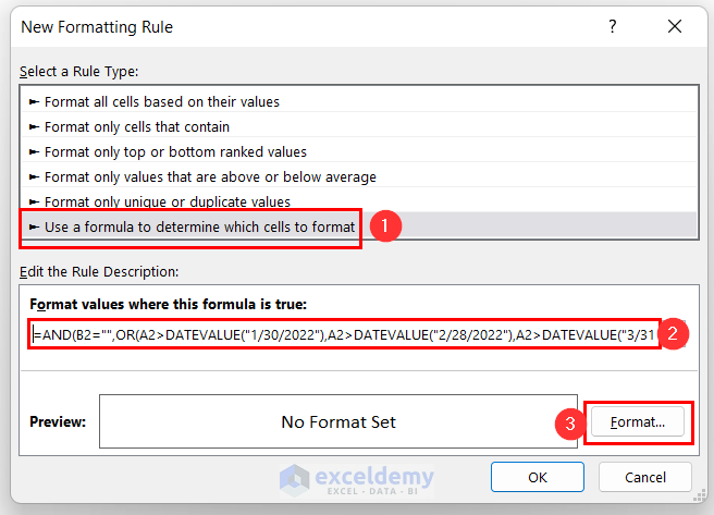
• In the opening dialog box, choose the indicated option and then type the following formula in the box
=AND(B2=””,OR(A2>DATEVALUE(“1/30/2022”),A2>DATEVALUE(“2/28/2022”),A2>DATEVALUE(“3/31/2022”)))
• Click on Format
• In the Format Cells dialog box go to the Fill tab >> select your desired color >> press OK.
Then, the following result will appear.