How to Create Drill Down Chart in Excel (with Easy Steps)

If you want to navigate through multiple levels or categories of a dataset, then Drill Down Chart is the best possible option for you. In Excel, it is very handy to drill down through a chart by following some simple steps. In this article, I have shown how to create a Drill Down Chart in Excel in a very simple way. Let’s get started.

Download Practice Workbook

You may download the following Excel workbook for better understanding and practice it yourself.

What Is a Drill Down Chart in Excel?

Some data charts contain multiple fields, and it is difficult to understand the chart if all the fields are shown at once. In this case, we need to Drill Down through the chart. A Drill Down chart is a type of chart or graph that allows the viewer to navigate through multiple levels of detail or data. It typically starts with an overview of the data at a high level, and then allows the user to drill down into more specific categories or subsets of the data.

How to Create Drill Down Chart in Excel (Step-by-Step Procedures)

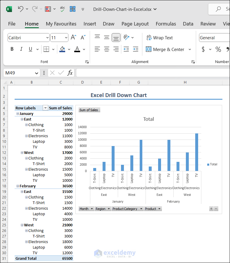
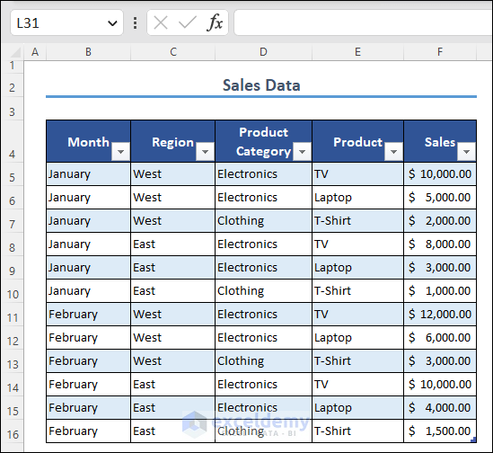
Suppose I have a dataset where I have sales data for 2 months. For each month, there are two regions – East and West. There are two categories of products- Electronics and Clothing. Again, in the Electronics category, there are two products- TV and Laptop. In the Clothing category, there is one product- T-shirts. I want to see the sum of sales for every category or level. So here, I will use Pivot Table to organize the data, and later, I will create a Pivot Chart following a drill down the chart.

1^st Step: Create a Pivot Table 

• To begin, select the cell in another sheet where you want to get the Pivot Table.
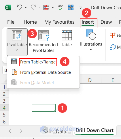
• Next, click on the Insert tab.
• Click on PivotTable and choose the From Table/Range option.

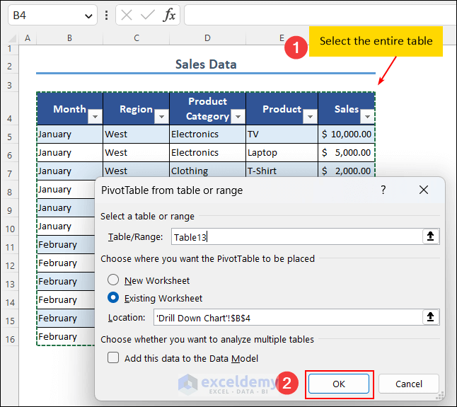
• You can see, PivotTable from table or range dialog box has appeared.
• Select the entire table of the dataset for which you want to create the Pivot Table.
• In Choose where you want the PivoTable to be Placed, select Existing Worksheet.
• Then, press OK.

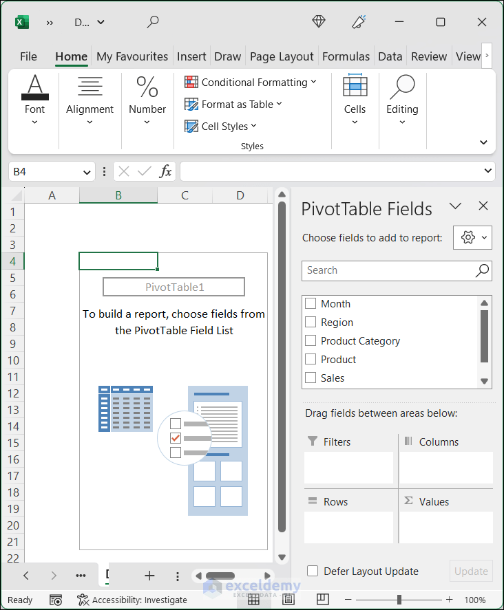
In the selected sheet, a PivotTable like the following image will appear, which is incomplete. You have to choose the fields of the dataset.

• In the PivotTable Fields Pane, put a tick beside the fields for which you want the PivotTable. Here, I have selected all the fields.
• You will notice that the field that contains values will automatically be placed below Values. It is named the Sum of Sales.
• The other fields will be placed below the Rows.

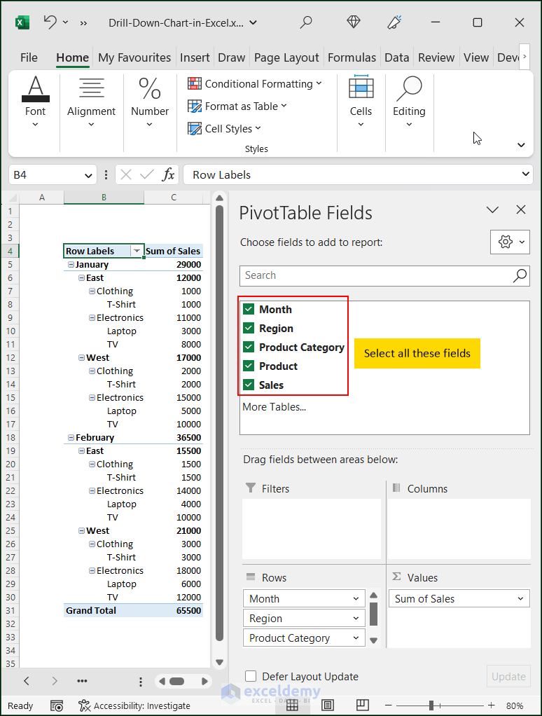
• Therefore, you have successfully created the Pivot Table.

Read More: How to Create Drill Down in Excel (with Easy Steps)

Similar Readings

• How to Insert Clipart in Excel (4 Easy Ways)
• Create Double Entry Bookkeeping in Excel
• How to Create Butterfly Chart in Excel (2 Easy Methods)
• Calculate Bootstrapping Spot Rates in Excel (2 Examples)
• How to Create an Organizational Chart in Excel from a List

2^nd Step: Create a Pivot Chart

The next step is to create a Pivot Chart for the newly created Pivot Table. Follow the steps below:

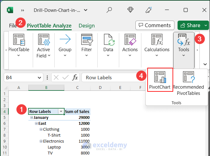
• Firstly, click on the Insert tab.
• Then, select PivotChart, and from the options that appear below, choose PivotChart.

• An Insert Chart dialog box will pop up.
• From All Chart, I have selected the Column chart. You can choose according to your dataset.
• Afterward, hit the OK button.

• So you have created the Pivot Chart for the selected Pivot Table.

Read More: How to Drill Down in Excel Without Pivot Table (With Easy Steps)

3^rd Step: Click on Drill Down Buttons in the Pivot Chart

In this step, you will learn how to drill down through the chart. It is really useful to know the sum of Sales for each field.

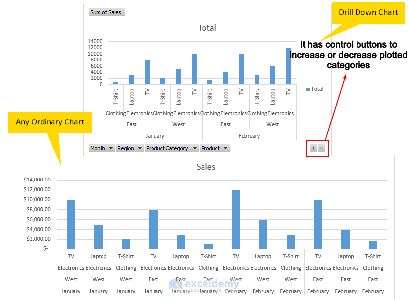
• You can see a small + and – sign icon at the bottom right corner of the Pivot Chart.
• This is the Drill down menu of the chart. If you want to see a detailed view, you have to click on the “ +” sign. and if you want to see less, then click on the “ –” sign.

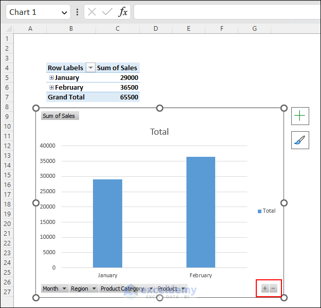
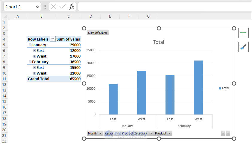
• Click on the “+” sign, and for each month, you can see both the East and West Region’s total sales data.

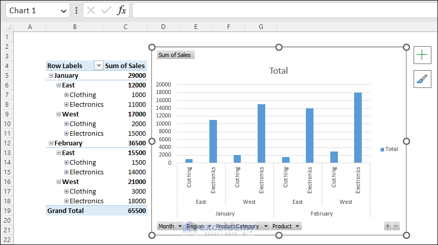
• Click one more time on the “+” sign, and you can see the total sales for the Product Categories.

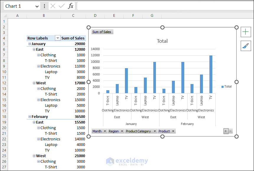
• Do the same action to see a more detailed view of the sum of sales for each field.

Here is a short video that will help you better understand.

Frequently Asked Questions

• What does Drill Down mean in Excel?

Answer: In Excel, “Drill Down” refers to the process of exploring and analyzing data in greater detail by breaking it down into smaller parts or subsets.

When you drill down on a particular set of data, you are essentially narrowing your focus to a more specific level. For example, if you have a summary table of sales data by year and quarter, you can drill down to see the sales data for a specific quarter or month.

To drill down in Excel, you can double-click on a cell or right-click and select “Drill Down” from the context menu. Excel will then display a new worksheet or pivot table that shows the underlying data that makes up the selected cell.

• Can I drill down in Excel pivot charts using no VBA?

Answer: Yes, you can drill down in Excel pivot charts without using VBA (Visual Basic for Applications). Excel pivot charts allow you to interactively explore and analyze data by drilling down into the details. Here’s how you can do it:

Use the “Expand” and “Collapse” buttons: Pivot charts also provide “Expand” and “Collapse” buttons that allow you to drill down or roll up the data in the chart. These buttons are available for certain chart types, such as pivot bar charts, pivot column charts, and pivot line charts. You can use these buttons to dynamically expand or collapse data categories, helping you to further explore and analyze the data.

Conclusion

This article provides a clear understanding of how to create a drill down chart in Excel. I have explained how to create a drill down chart in 3 easy steps. I hope this article will help you navigate through the subsets of your dataset. If you have any questions regarding this article, please leave a comment so that we can help.

Related Articles

• How to Show Menu Bar in Excel (2 Common Cases)
• Use of Task Pane in Excel (Detailed Analysis)
• How to Change 1000 Separator to 100 Separator in Excel
• Show Full Cell Contents on Hover in Excel (5 Quick Ways)
• How to Check If Value Is Between 10 and 20 in Excel
• Mark Workbook as Final in Excel (with Easy Steps)
• How to Move Data from Row to Column in Excel (4 Easy Ways)