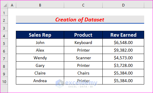
Step 1 – Create a Dataset with Proper Parameters
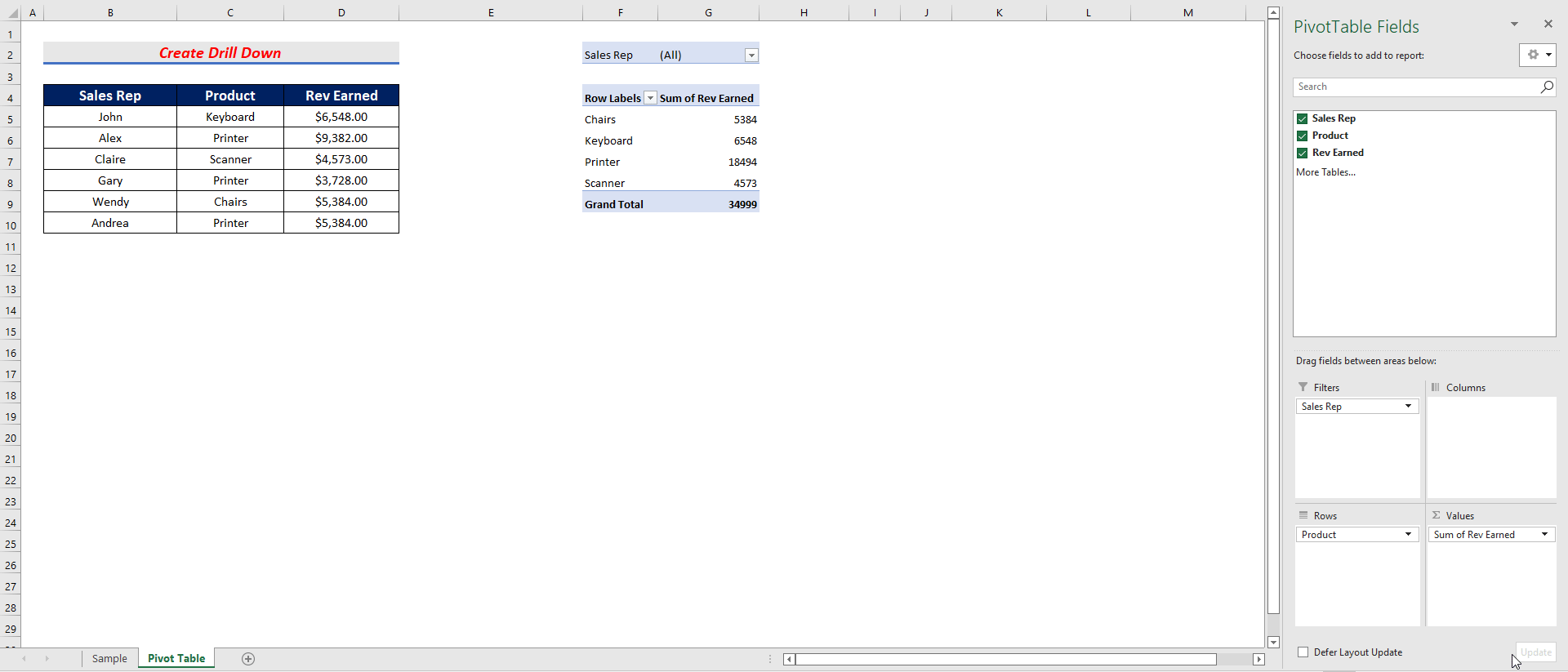
Create your dataset in Excel. We created a column of Sales Representatives names with two other columns of Product and Revenue Earned. Our dataset looks as shown below.
Read More: How to Drill Down in Excel Without Pivot Table (With Easy Steps)
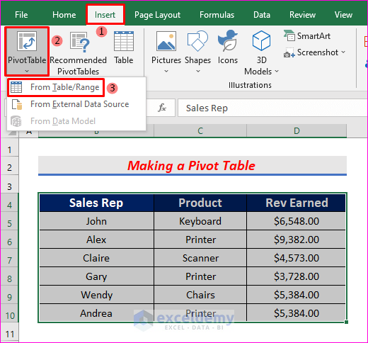
Step 2 – Insert a Pivot Table
We need to insert a pivot table from the created dataset.
- Select the whole table. From your Insert tab, go to,
Insert → Pivot Table → From Table/Range
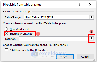
- Once you select From Table/Range, a window will pop up.
- If you want your pivot table in the same worksheet, select Existing Worksheet.
- Click on the arrow to choose Location.
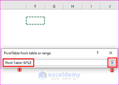
- Select the cell where you want your pivot table and click on the arrow.
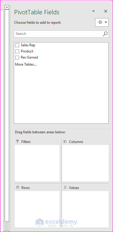
- Press Enter and the Pivot Table Fields will be inserted on the right side of your worksheet.
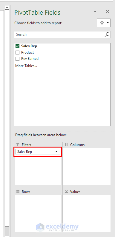
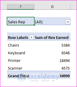
- From the Pivot Table Fields, drag Sales Rep and drop it down to the Filters area.
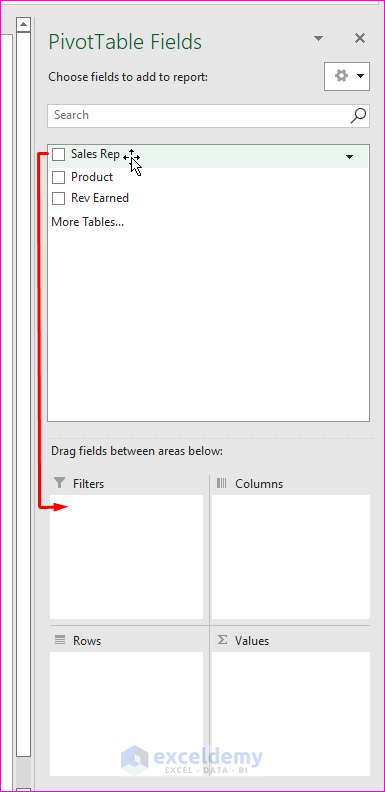
- You will find Sales Representatives in the Filters area.
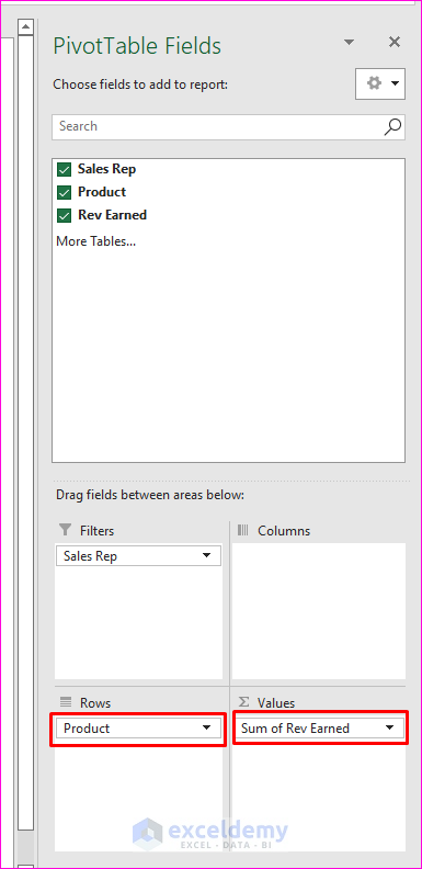
- Drag Product under the Rows area and Revenue Earned in the Values area.
- The pivot table will be in the worksheet.
Read More: How to Create a Calculator Using Macros in Excel (with Easy Steps)
Similar Readings
- How to Insert Clipart in Excel (4 Easy Ways)
- Create Double Entry Bookkeeping in Excel
- How to Write X Bar in Excel (3 Easy Ways)
- Calculate Bootstrapping Spot Rates in Excel (2 Examples)
Step 3 – Create Drill Down in Excel
- Double-click on any of the Rev Earned data.
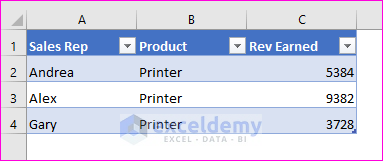
- It will open a new worksheet with the drilled down data.
- We double clicked on the Rev Earned of Printer and all data with the Printer column opened up in another worksheet. Look at the below GIF to understand the procedures.
- You can also move your cursor on the data and click the right button of your mouse and then select Show Details.
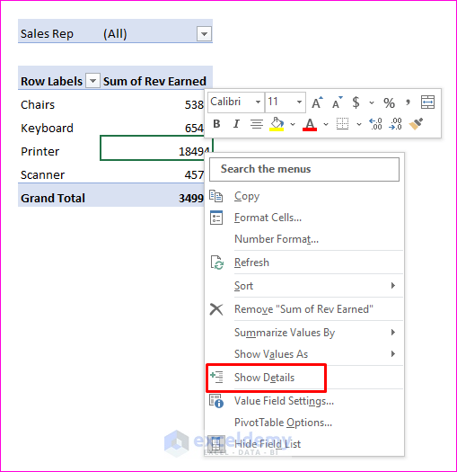
- It will create a new worksheet and you will have your drilled-down data in there.
Notes
- Pivot tables arrange data alphabetically by default. If you want to rearrange the data, you can use the Sort option.
- If you want to create your pivot table in a new worksheet, select New Worksheet from Pivot Table from table or range pop-up box.
Read More: How to Fix Formula in Excel (9 Easy Methods)
Related Articles
- How to Show Menu Bar in Excel (2 Common Cases)
- Use of Task Pane in Excel (Detailed Analysis)
- How to Change 1000 Separator to 100 Separator in Excel
- Show Full Cell Contents on Hover in Excel (5 Quick Ways)
- How to Check If Value Is Between 10 and 20 in Excel
- Mark Workbook as Final in Excel (with Easy Steps)
- How to Move Data from Row to Column in Excel (4 Easy Ways)

