Step 1 – Record Macro
Steps:
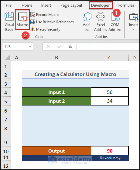
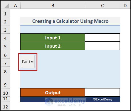
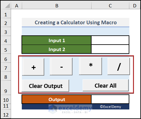
- Create a basic outline as shown in the following image. We constructed two Input cells in cells C4 and C5. You can seeOutput cell in cell C10.
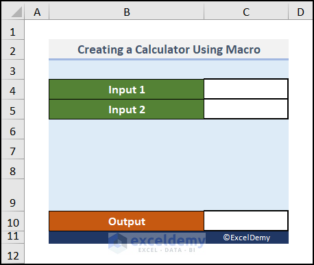
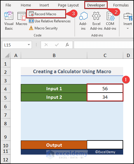
- Enter some dummy values in cells C4 and C5.
- Go to the Developer If the Developer tab isn’t available on the ribbon, go to, How to show Developer Tab in Excel.
- Click on Record Macro in the Code group of commands.
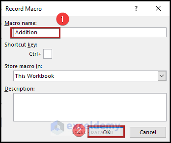
The Record Macro dialog box will open.
- In the Macro name box, enter Addition.
- Click OK.
Excel will record the works done in the worksheet.
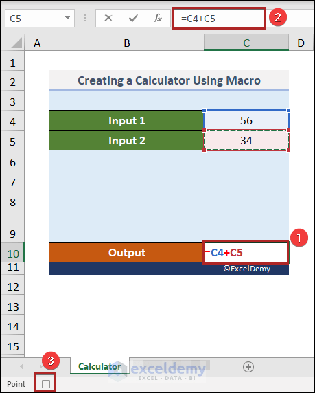
- Select cell C10 and enter the following formula.
=C4+C5- Press ENTER.
- Click on the Stop button on the left-bottom corner of the display to stop recording the macro.
Step 2 – Copy Code for Various Operations
Steps:
- Proceed to the Developer
- Click on Macros in the Code
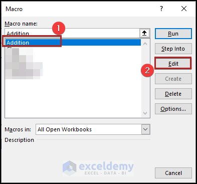
The Macro dialog box will pop up.
- Select the Addition macro.
- Click Edit.
The Microsoft Visual Basic for Applications window will open. We can see the relevant codes here.
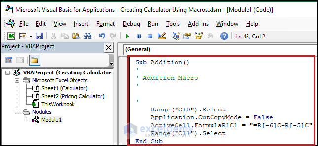
Follow this sub-procedure to create macros for other operations like subtraction, multiplication, and division.
- Copy the code and paste it three times.
- Change the operator from (+) to (–) for subtraction, to (*) for multiplication and to (/) for division.

We chose to create 2 dedicated macros for deleting contents from the cells.
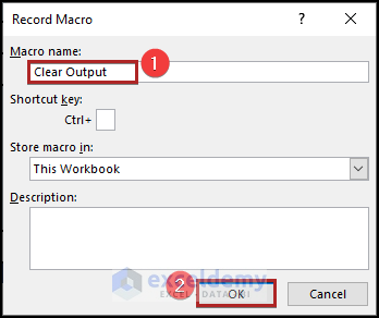
- Open the Record Macro dialog box.
- Enter Clear_Output as the Macro name.
- Click OK.
The macro will start recording.
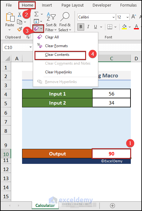
- Select cell C10.
- Navigate to the Home tab.
- Click on the Clear drop-down icon.
- Select Clear Contents.
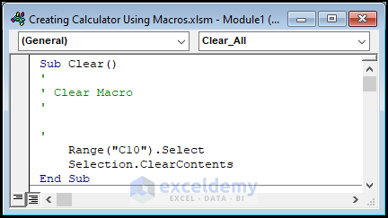
- Click on the Stop button on the Status Bar.
You can see the VBA code for this macro.
- We created a different macro to Clear_All.
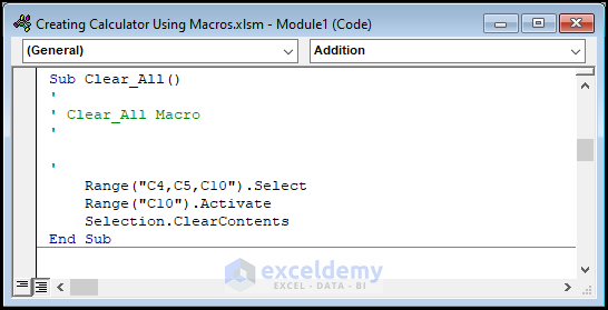
With this macro, we can delete the contents in cells C4, C5, and C10.
Step 3 – Insert Button from Form Controls
Steps:
- Go to Developer.
- Click on Insert.
- Choose Button (Form Control).
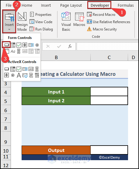
- Place a button as shown in the image below.
- Right-click on the button and click on the Edit Text option.
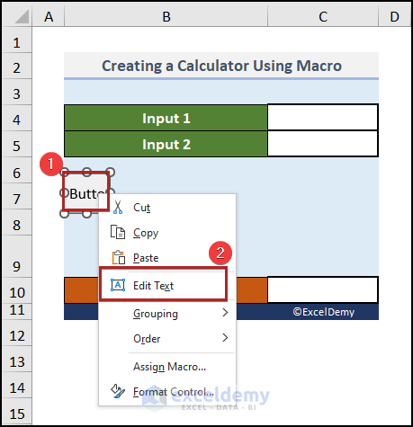
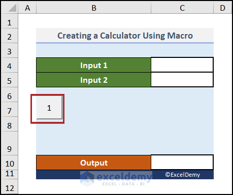
The button for Addition is created.
Step 4 – Assign Macro to Button
Steps:
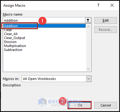
- Right-click on the button and select Assign macro… from the context menu.
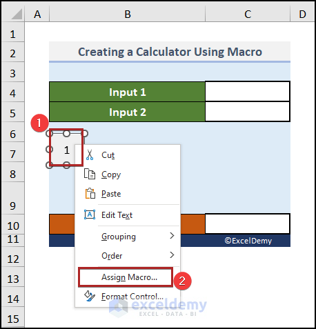
- From the Assign Macro dialog box, select Addition in the Macro name box.
- Click OK.
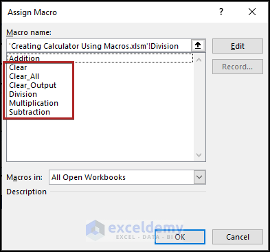
- Follow the previous steps to assign macros to their respective buttons.
- Moreover, follow the previous steps to assign macros to their respective buttons.
Check whether it is working or not.
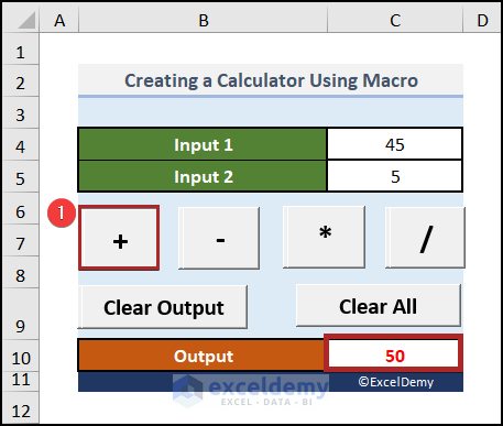
- Enter two inputs in cells C4 and C5.
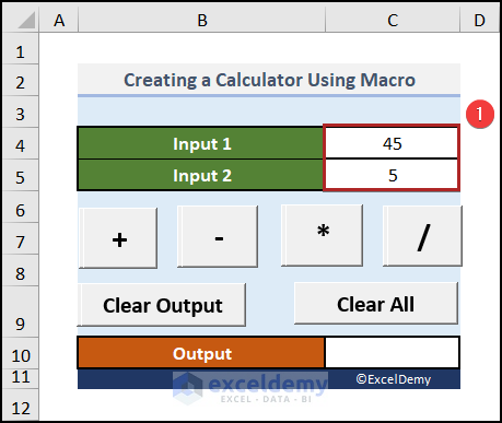
- Click on the + (plus) button to get the output in cell C10.
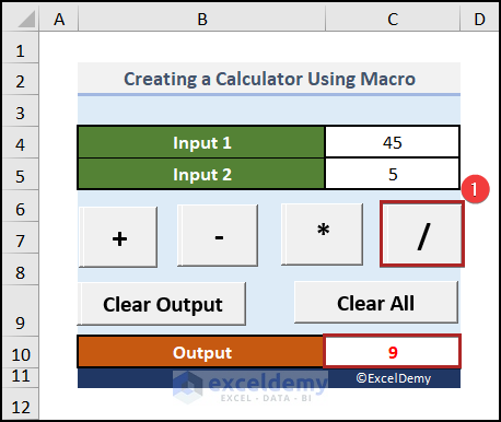
- Click on the/ (division) button to get the result in cell C10.
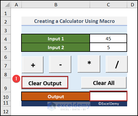
To clear the output in cell C10, click on the Clear Output button.
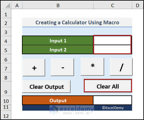
The Clear All button will delete the inputs and outputs.
Read More: How to Create Toggle Button on Excel VBA UserForm
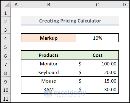
How to Create a Pricing Calculator in Excel
This is how to calculate the selling price of a product based on its cost and %markup. If we have the Cost and our expected %Markup the formula for calculating the Selling Price would be:
Steps:
The sample dataset below constains a list of some Products and their corresponding production Costs in columns B and C. We have the expected Markup percentage in cell C4, which is 10%.
- Create a new column with the heading Selling Price under Column D.
- Enter the following formula in cell D7.
=C7*(1+$D$4)- Press ENTER.
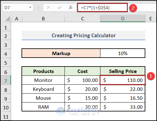
Enter your expected Markup percentage in cell D4 and your Costs in Column C. This calculator will calculate others.
Download Practice Workbook
Related Articles
- How to Use Excel VBA Userform
- Excel VBA: Create a Progress Bar While Macro Is Running
- How to Create Cascading Combo Boxes in Excel VBA User Form

