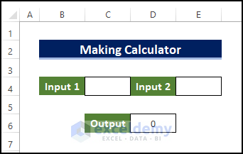
Step 1 – Create the Outline
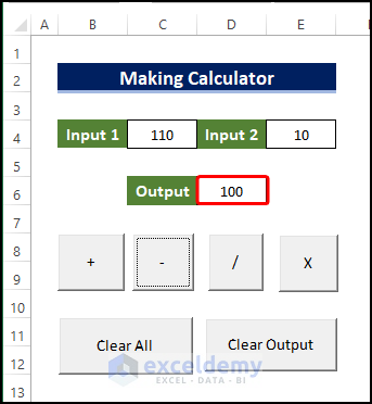
- We arranged the input and the output cells as shown below.
Read More: How to Create a Calculator Using Macros in Excel
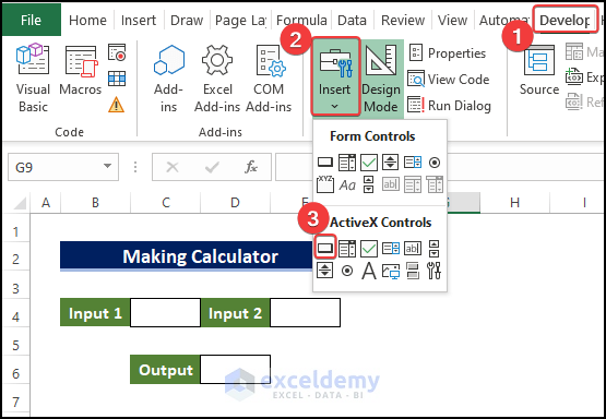
Step 2 – Input a Command Button
- Go to the Developer tab.
- Select Insert.
- Choose a Command Button from ActiveX Control.
- Click and drag with the cursor to draw the shape of your Command Button box.
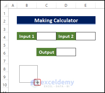
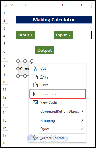
- We’ll get a basic command button with a default caption.
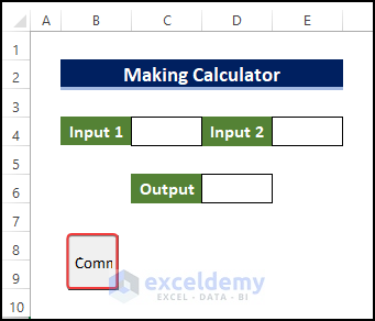
- Right-click on the box and select Properties from the context menu.
- Click on the Caption and put “+”.
- Close the Properties dialog.
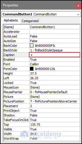
- The command button is now present with a modified caption.

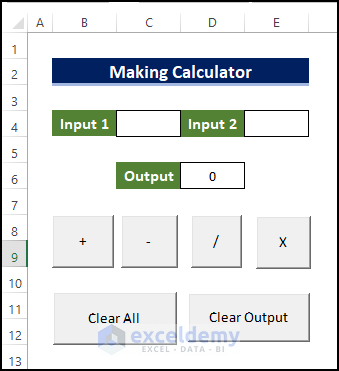
- Repeat the process for the rest of the buttons as shown below.
- The different buttons will denote different operations.
- Clear All button will clear everything(the inputs and outputs)
- Clear Output will clear only the output value so that you can restart the operation immediately.
Step 3 – Create VBA Macro and Attach to the Buttons
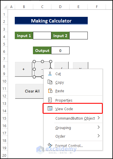
- Right-click on the first button and select View Code from the context menu.
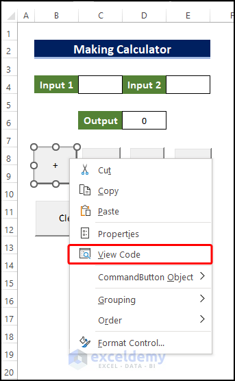
- Insert the following code in the code editor.
Private Sub CommandButton1_Click()
Range("D6") = Range("C4").Value + Range("D6").Value + Range("E4").Value
End Sub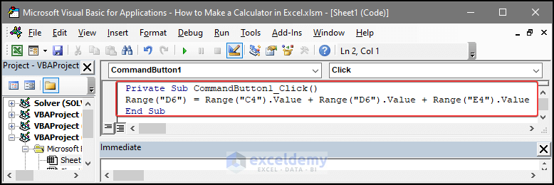
- Move on to the next button “-”.
- Right-click on it and select View Code from the context menu.
- Insert the following code:
Private Sub CommandButton3_Click()
If Range("D6").Value = 0 Then
Range("D6") = Range("C4").Value - Range("E4").Value
Else
Range("D6") = Range("D6").Value - Range("E4").Value
End If
End Sub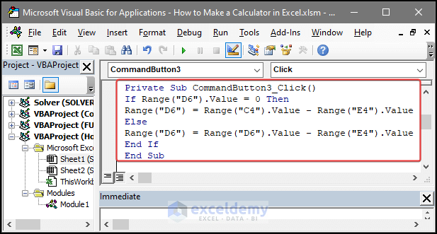
- Repeat the same procedure for the multiplication button with this code:
Private Sub CommandButton2_Click()
Range("D6") = Range("C4").Value * Range("E4").Value
End Sub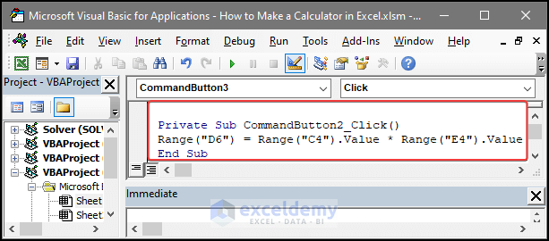
- Repeat the same procedure for the division button and enter this code for the button.
Private Sub CommandButton4_Click()
Range("D6") = Range("C4").Value / Range("E4").Value
End Sub- Repeat the same procedure for the Clear All button and enter the following code for that button.
Private Sub CommandButton5_Click()
Range("C4").ClearContents
Range("E4").ClearContents
Range("D6").ClearContents
End Sub- For Clear Output button, insert the code below:
Private Sub CommandButton6_Click()
Range("D6").ClearContents
End Sub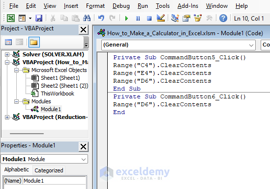
Step 4 – Test the Calculator
- Enter 110 and 10 as Input 1 and Input 2, respectively, in cells C4 and E4.
- Click on the “+” icon.
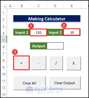
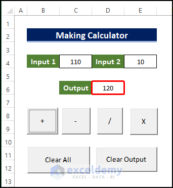
- You should get the result 120.
- Press the Clear Output option.
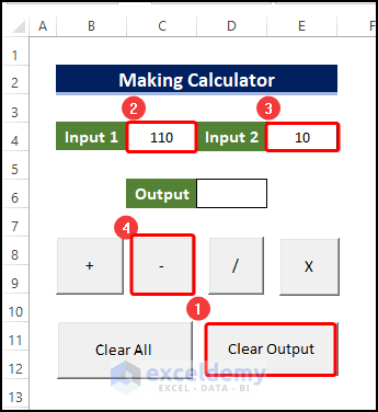
- Use the same values and press the – button.
- The output will be shown as 100 in cell D6.
Download the Template
Related Articles
- How to Use Excel VBA Userform
- Excel VBA: Create a Progress Bar While Macro Is Running
- How to Create Cascading Combo Boxes in Excel VBA User Form


FOLLOWED YOUR STEPS BUT IT DIDN’T WORK FOR ME – GIVES ME AN AMBIGUOUS NAME DETECTED:CLEARCELLS ERROR AND NONE OF THE BUTTONS WORK
Dear April
Thanks for your concern. There were some minor formatting issues with the VBA codes. Sorry for the inconvenience. We have updated our article. If you follow now, you will get the perfect calculator.
Thanks for your help
Regards,
Joyanta Mitra
ExcelDemy