As of now, Excel doesn’t have any built-in currency conversion tool yet. So we either need at least a basic multiplication formula or other formulas or a combination of those to convert currencies depending on how we are using them. This article will focus on currency conversion in Excel using the VLOOKUP function.
Currency Conversion Using VLOOKUP in Excel: 2 Suitable Examples
The VLOOKUP function or Vertical Lookup function is used to search for a certain value in a column or an array. It looks for a value in the leftmost column of a table and returns the specific column value you want from the same row. This function takes three primary arguments- a lookup value, a table array from where it is searching for the value, and the column index number it will return from the matching row. More details can be found in the examples.
The main purpose of using this function for currency conversion is to find the rate of currency changes from a different dataset and use it for multiplication or division- depending on your direction or conversion.
Two examples are included here for currency conversion in Excel Using VLOOKUP for a better understanding of the process.
1. Convert USD to Other Currencies Using VLOOKUP
In the first example, we are going to focus on the following dataset.
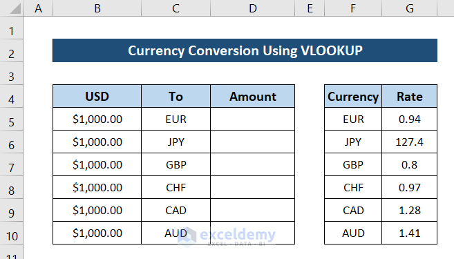
Here, you can see there is a dataset included on the right consisting of different currency rates when converted from US dollars. We are going to convert the amounts in US dollars in range B5:B10 to different currencies depending on the rows in range C5:C10. To do that, we are going to use the VLOOKUP function to find the rate from the dataset on the right.
Steps:
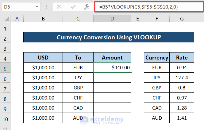
- First of all, select cell D5.
- Then write down the following formula in the cell.
=B5*VLOOKUP(C5,$F$5:$G$10,2,0)
- Now press Enter on your keyboard. You will have your first converted value.
- After that select the cell again. Finally, click and drag the Fill handle icon to the end of the column to fill the values for the rest of the column.
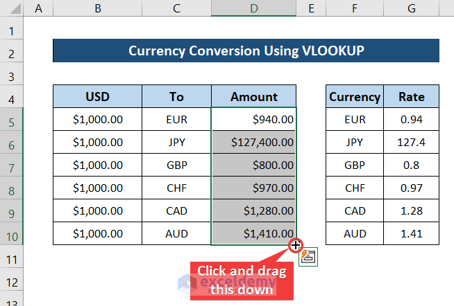
As a result, the currency conversion will be completed in Excel using the VLOOKUP function.
2. Currency Conversion Using Table in Excel
For the second example, we will focus on the following dataset to make a currency converter.

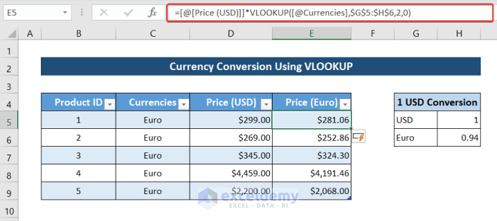
As you can see, this dataset has a table for the conversion rate too on the right of it. We will be using these values for the vertical lookup. And convert the main dataset into a table for currency conversion. Here, this example will also contain the VLOOKUP function.
Steps:
- First, select the dataset which you want to convert to a currency converter.

- Now press Ctrl+T on your keyboard to enter a table. Then click on OK.
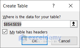
- As a result, the dataset will be converted into a table.

- Now go to cell E5 and write down the following formula.
=[@[Price(USD)]]*VLOOKUP([@Currencies],$G$5:$H$6,2,0)
- After that press Enter. This will convert the first value in the cell as well as the rest of the values in the column.
From now on you can also add a new row to the table and fill out the original values. And you will see that Excel automatically fills up the final column value with the formula and converts the currency. This is another way you can use the VLOOKUP function for currency conversion in Excel.
Alternative Methods of Currency Conversion without VLOOKUP in Excel
Unlike the previous examples where only the VLOOKUP function is used for currency conversion, you can use many more methods and formulas to do that in Excel. Here is a short glimpse of those methods.
1. Currency Conversion Using Multiplication
You can use the simple old-school multiplication of a currency with the conversion rate to find a new one easily in Excel. For a more detailed guide follow the steps.
We are using the following dataset for a demonstration.

We will be converting the USD values to Euro using the multiplication method. Cell C11 contains the rate value.
Steps:
- First of all, select cell C5.
- Then write down the following formula in the cell.
=B5*$C$11

- Now press Enter on your keyboard.

- After that, select the cell again. And then click and drag the Fill handle icon to fill out the rest of the column with the formula.
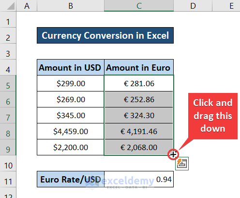
As a result, you will have the currency converted from USD to Euro.
2. Currency Conversion Using Nested IF Formula
You can also use the IF function to replicate a substitute for the VLOOKUP function. More accurately, a nested IF formula. This formula of a nested IF function is a bit lengthy and repetitive. So use this function only if the convertible currencies are limited to a few.
The IF function takes a condition as the first argument and checks if the condition is true or false. It takes another mandatory argument which it returns if the condition is true. The function can take another argument that it returns in case the condition is false. We will use the last argument as another IF function to go through all the currencies for conversion.
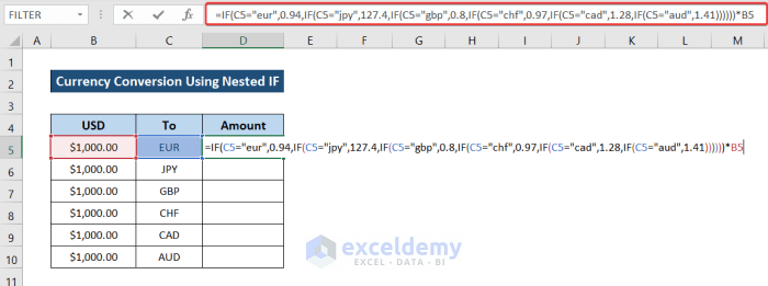
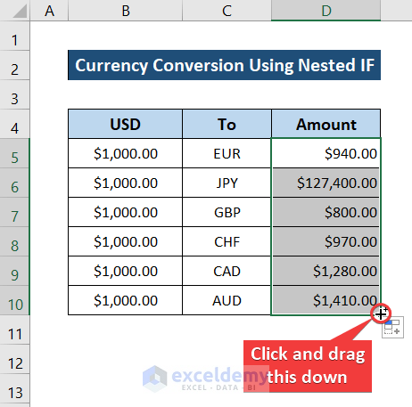
For demonstration, we are using the following dataset.

Steps:
- First, go to cell D5.
- Now write down the following formula in the cell.
=IF(C5="eur",0.94,IF(C5="jpy",127.4,IF(C5="gbp",0.8,IF(C5="chf",0.97,IF(C5="cad",1.28,IF(C5="aud",1.41))))))*B5
- Then press Enter on your keyboard. As a result, you will have the first value converted.
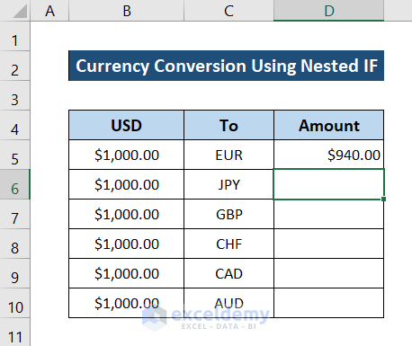
- Now select the cell again. Finally, click and drag the Fill handle icon to fill out the rest of the column with the formula for their respective cells.
Thus you can perform currency conversion with a nested IF formula in Excel.
🔍 Breakdown of the Formula
👉 The IF(C5=”eur”,0.94,…) checks if the value of the cell is equal to the string “eur” or not. If it is, then it returns the value 0.94.
👉 And if the condition is not met, it moves on to the next IF function, which is IF(C5=“jpy”,...). If the condition is met here, it returns the value 127.4.
👉 If not, then the formula moves on to the next function IF(C5=“gbp”,0.8,…). This function returns the value of 0.8 if the condition is met.
👉 Otherwise moves on and enters a new function IF(C5=“chf”,0.97,…). If the value in it is now indeed “chf” then it now returns 0.97.
👉 Else, it moves onto the next portion IF(C5=”cad”,1.28,…) and tests the condition. If it is true now, the function returns the value 1.28.
👉 IF(C5=”aud”,1.41) comes into play if none of the above conditions is met and returns 1.41 if the value in the cell is “aud”. At this point, if it still doesn’t match, then it returns nothing.
👉 If any of the conditions are met in the above functions, it returns the matching conversion rate and finally multiplies that with the original value. And finally, the whole function returns the converted value.
3. Combination of INDEX and MATCH Functions in Excel
There is another way to replicate the VLOOKUP function in Excel for currency conversion. It is a combination of the INDEX and MATCH functions.
The INDEX function takes an array and the row number of the array as arguments and returns the value of the next column, which it can also take as an optional argument. While the MATCH function takes a lookup value and a lookup array as its primary arguments. It can also take an optional argument depending on whether you want an exact, less than, or greater than match. The function returns the position of the matched value.
As a result, we can use the MATCH function to find a currency match and then the INDEX function to find out the value of that position to mimic the operation of the VLOOKUP function.
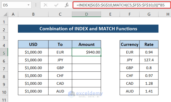
To demonstrate the process, we are using the following dataset.

Steps:
- First, select cell D5.
- Second, write down the following formula in the cell.
=INDEX($G$5:$G$10,MATCH(C5,$F$5:$F$10,0))*B5
- Now press Enter on your keyboard.
- After that, select the cell again. Then click and drag the fill handle icon to fill out the rest of the column with the formula.
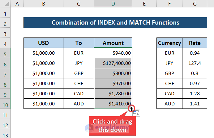
This will also convert currencies in Excel. But this time with a combination of the INDEX and MATCH functions.
🔍 Breakdown of the Formula
👉 The MATCH(C5,$F$5:$F$10,0) function matches the value of cell C5 within the array F5:F10 and returns the first position of the exact match. Here it returns 1.
👉 INDEX($G$5:$G$10, MATCH(C5,$F$5:$F$10,0)) portion of the formula returns the value of the index where the previous function matched. As the value was 1, it returns the conversion rate of 0.94 here.
👉 Finally, INDEX($G$5:$G$10, MATCH(C5,$F$5:$F$10,0))*B5 multiplies the conversion rate with the original amount and returns the result.
Download Practice Workbook
You can download the workbook containing all the datasets, currency values, and results below. Try yourself with the example as you go through the article.
Conclusion
These were the different methods you can use for currency conversion in Excel using both the VLOOKUP function and other formulas. Hope you have found this guide helpful and informative. If you have any questions or suggestions, let us know below.
<< Go Back to Currency Conversion in Excel | Learn Excel
Get FREE Advanced Excel Exercises with Solutions!
