When we use the Excel VLOOKUP function, we have to input the Column number from which it’ll return the data. But, manually counting the column number from a large worksheet is an inconvenient process. It can also result in errors. In this article, we will show you the simple methods to Count Columns for VLOOKUP in Excel.
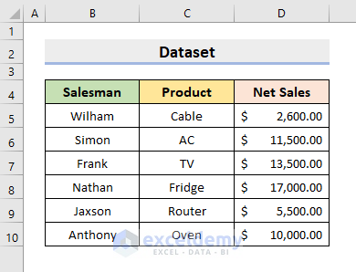
To illustrate, I’m going to use a sample dataset as an example. For instance, the following dataset represents the Salesman, Product, and Net Sales of a company.
Introduction to Excel VLOOKUP Function
- Syntax
VLOOKUP(lookup_value, table_array, col_index_num, [range_lookup])
- Arguments
lookup_value: The value to look for in the leftmost column of the given table.
table_array: The table in which it looks for the lookup_value in the leftmost column.
col_index_num: The number of the column in the table from which a value is to be returned.
[range_lookup]: Tells whether an exact or partial match of the lookup_value is required. 0 for an exact match, 1 for a partial match. Default is 1 (partial match). This is optional.
How to Count Columns for VLOOKUP in Excel: 2 Methods
1. Count Columns with COLUMN Function for VLOOKUP in Excel
Excel provides many Functions and we use them for performing numerous operations. The COLUMN function is one of those useful functions. It helps us to find out the column number of a reference. Thus we don’t have to count manually to get the column number. In our first method, we’ll use the COLUMN function to Count Columns for VLOOKUP in Excel. Therefore, follow the steps below to perform the task.
STEPS:
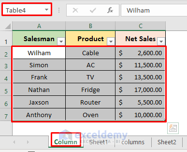
- First, we have a source table: Table4 in the Column From here, we’ll pick up our desired values and place them in Sheet1 by creating a formula.
- Then, in Sheet1, select cell C2 and type the formula:
=VLOOKUP(A2,Table4,COLUMN(Table4[Net Sales]),FALSE)- Afterward, press Enter.

Here, the COLUMN function automatically counts the column number of the column Net Sales in Table4. After that, the VLOOKUP function looks for the A2 cell value in Table4 and returns the value present in the column Net Sales.
- Finally, use the AutoFill tool to complete the series.

2. Excel COLUMNS Function to Count Last Column for VLOOKUP
However, if we want to return cell values present in the last column of any data range, we can simply use the Excel COLUMNS function in the VLOOKUP argument. The COLUMNS function counts the total number of columns in a given reference. So, learn the below process to Count the Last Column for VLOOKUP and return the value.
STEPS:
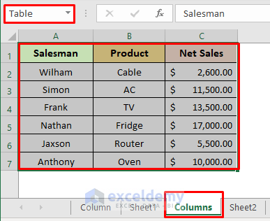
- Firstly, we have the Table in sheet Columns as our source.
- Now, select cell C2 in Sheet2. Type the formula:
=VLOOKUP(A2,Table,COLUMNS(Table),FALSE)- After that, press Enter.
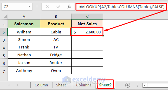
Here, the COLUMNS function counts the number of columns present in Table. Subsequently, the VLOOKUP function searches for A2 in Table and returns the value from the last column.
- Lastly, fill the rest with the AutoFill tool.

Things to Remember
- To avoid errors while using the COLUMN and COLUMNS functions, you should start your dataset from the leftmost column.
- You should input FALSE for an exact match in the VLOOKUP argument. Otherwise, it may return the wrong values.
Download Practice Workbook
Conclusion
Henceforth, you will be able to Count Columns for VLOOKUP in Excel with the above-described methods. Keep using them and let us know if you have any more ways to do the task. Don’t forget to drop comments, suggestions, or queries if you have any in the comment section below.
<< Go Back to Count Columns | Formula List | Learn Excel
Get FREE Advanced Excel Exercises with Solutions!
