How to Construct Cost Inflation Index Calculator in Excel

Undoubtedly, Microsoft Excel is a ubiquitous tool for analyzing data and solving complex problems. Now, wouldn’t it be great if we could make a calculator for inflating costs? Sounds complex, right? Wrong! In this article, we’ll demonstrate the detailed procedure on how to construct cost inflation index calculator in Excel. In addition, we’ll also learn to use the cost inflation index to reduce taxes on capital gains and plot the cost inflation index chart.

The animated GIF above is an overview of this article, which represents the construction of a cost inflation index calculator in Excel. In the following sections, we’ll learn what the cost inflation index is and the steps to make a cost inflation index calculator with the necessary illustrations.

What Is Cost Inflation Index?

First and foremost, let’s start with a quick explanation, so you don’t have to spend all day on this.
Simply put, the Cost Inflation Index is a tool for measuring inflation when computing the capital gains of assets in the long run. Since assets tend to appreciate in value over time, the owner can earn a large capital gain (difference between the selling and acquisition prices) when selling this asset.
In general, capital gains are subjected to taxes by the government. In fact, the cost inflation index helps to reduce this tax by adjusting the purchase price of the asset with the cost inflation index. Thus, decreasing the net profit and hence the capital gains tax.

How to Construct Cost Inflation Index Calculator in Excel: 3 Easy Steps

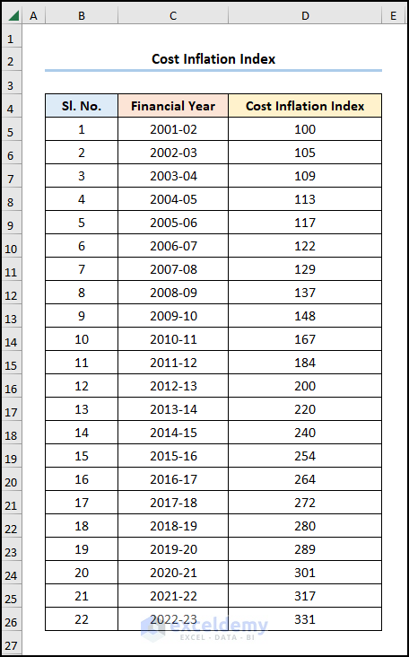
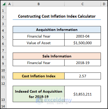
To begin with, let’s consider the Cost Inflation Index table shown in the B4:B26 cells containing the “Sl. No.”, “Financial Year”, and “Cost Inflation Index” columns respectively.

Here, we want to obtain the indexed cost of acquisition for a specific year by combining the VLOOKUP and IFERROR functions to look up the “Cost Inflation Index” value for the corresponding “Financial Year”. So, let’s see it in action.

Here, we have used the Microsoft Excel 365 version; you may use any other version at your convenience.

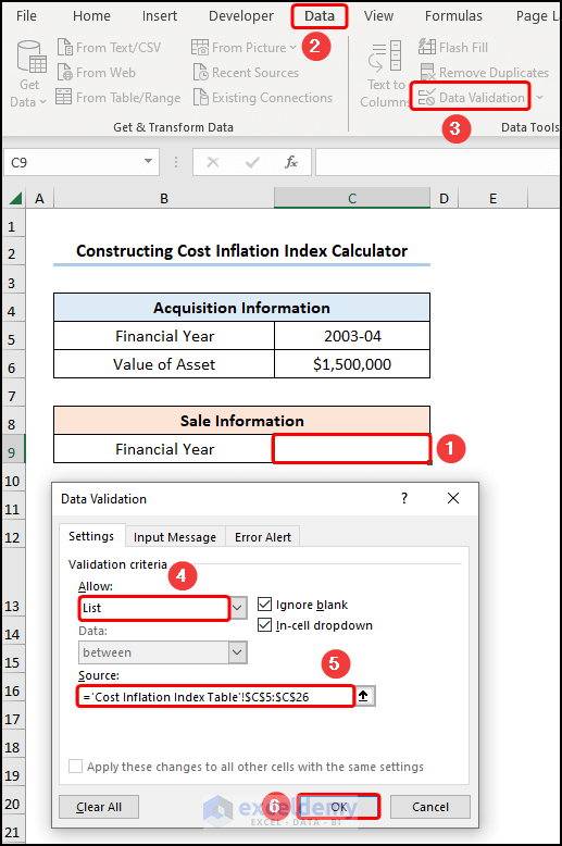
📌 Step 1: Make Drop-down for Financial Years with Data Validation

First, go to the C5 cell >> move to the Data tab >> click the Data Validation drop-down >> choose the Data Validation option.

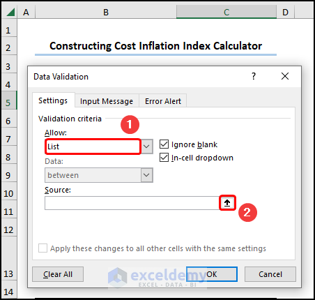
Now, this opens the Data Validation dialog box.

Next, in the Allow field, select the List option >> click the Arrow button.

Then, highlight the C5:C26 cells as the Source for the drop-down.

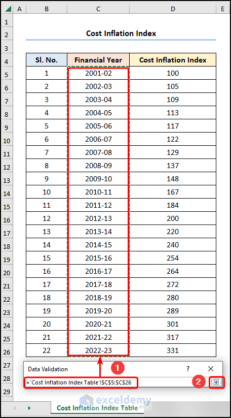
Afterward, press OK to close the Data Validation window.

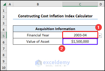
After that, choose a “Financial Year” (“2003-04”) in the “Acquisition Information” table >> enter the “Value of Asset” (“$1,500,000”) in the C6 cell.

In the same manner, insert a second drop-down list for the “Sale Information”.

📌 Step 2: Obtain Cost Inflation Index Using VLOOKUP Function

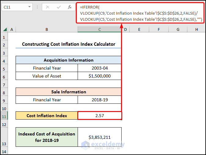
Second, jump to the C11 cell >> enter the following equation >> press ENTER.

=IFERROR(VLOOKUP(C9,'Cost Inflation Index Table'!C5:$D$26,2,FALSE)/VLOOKUP(C5,'Cost Inflation Index Table'!C5:$D$26,2,FALSE),"")

Formula Breakdown

VLOOKUP(C9,’Cost Inflation Index Table’!C5:$D$26,2,FALSE) → looks for a value in the left-most column of a table, and then returns a value in the same row from a column you specify. Here, C9 cell ( lookup_value argument) is mapped from the ‘Cost Inflation Index Table’!C5:$D$26(table_array argument) array in the “Cost Inflation Table” worksheet. Next, 2 (col_index_num argument) represents the column number of the lookup value. Lastly, FALSE (range_lookup argument) refers to the Exact match of the lookup value.
- Output → 280
VLOOKUP(C5,’Cost Inflation Index Table’!C5:$D$26,2,FALSE) → here, C5 cell ( lookup_value argument) is mapped from the ‘Cost Inflation Index Table’!C5:$D$26(table_array argument) array in the “Cost Inflation Table” worksheet. Next, 2 (col_index_num argument) represents the column number of the lookup value. Lastly, FALSE (range_lookup argument) refers to the Exact match of the lookup value.
- Output → 109
IFERROR(VLOOKUP(C9,’Cost Inflation Index Table’!C5:$D$26,2,FALSE)/VLOOKUP(C5,’Cost Inflation Index Table’!C5:$D$26,2,FALSE),””) → becomes
- IFERROR(280/109,””) → returns value_if_error if the expression has an error and the value of the expression itself otherwise. Here, 280/109 is the value argument, and “” is the value_if_error argument. In this case, the function returns the result of the division.
- Output → 2.57

📃 Note: Please make sure to use Absolute Cell Reference by pressing the F4 key on your keyboard.

📌 Step 3: Calculate Indexed Cost of Acquisition

Third, proceed to the C13 cell >> insert the expression into the Formula Bar.

=IFERROR(C6*C11,"")

Here, the IFERROR function checks whether the product of the C6 and C11 cells is valid, in which case it returns the result; otherwise, it returns blank.

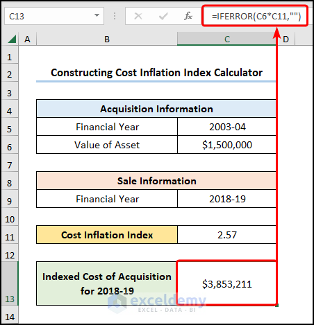
Finally, the results should look like the image shown below.

How to Use Cost Inflation Index to Reduce Taxes on Capital Gains

For one thing, we can introduce some modifications to our cost inflation index calculator to compute the tax savings on capital gains. It’s quick and simple, so just follow the steps shown below.

📌 Steps:

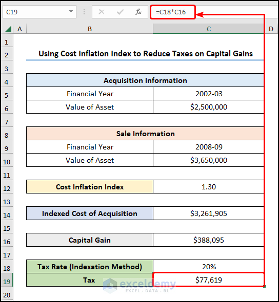
Initially, follow the steps shown previously to get the Indexed Cost of Acquisition shown in the picture below.

Following this, go to the C16 cell >> subtract the value of the C14 cell from the C10 cell >> click on ENTER.

=C10-C14

For instance, the C10 and C14 cells refer to the “Value of Asset” and “Indexed Cost of Acquisition”.

Not long after, calculate the “Tax Rate” for the indexation method in the C19 cell.

=C18*C16

For example, the C16 and C18 cells point to the “Capital Gain” and the given “20% Tax Rate”.

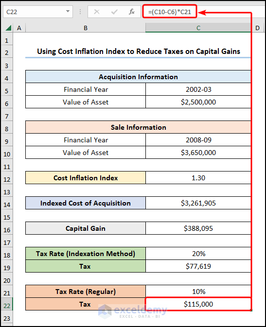
At this point, copy and paste the formula into the C22 cell >> press ENTER to obtain the “Regular Tax Rate”.

=(C10-C6)*C21

On this occasion, the C6 and C10cells indicate the “Value of Asset” in the “Acquisition and Sale Information” tables, while the C21 cell represents the “Regular Tax Rate of 10%”.

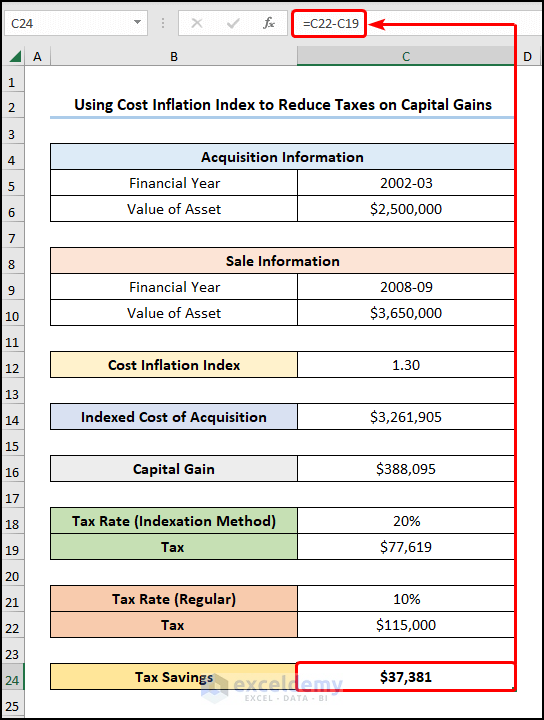
Lastly, we can return the “Tax Savings” using the formula given below.

=C22-C19

Here, the C19 and C22 cells represent the “Indexed Tax” and the “Regular Tax”.

How to Make Cost Inflation Index Chart in Excel

Last but not least, we can also make a cost inflation index chart using Excel’s powerful graphing engine. Now, allow us to demonstrate the process in the steps below.

📌 Steps:

In the first place, choose the D5:D26 cells >> navigate to the Insert tab >> insert 2-D Column chart.

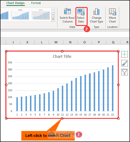
In turn, left-click to select the chart >> press the Select Data button.

Now, in the Select Data Source window, press the Edit button.

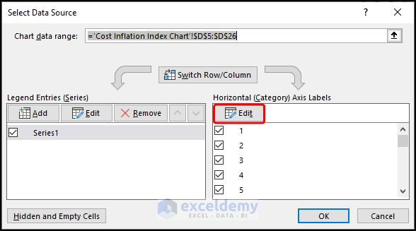
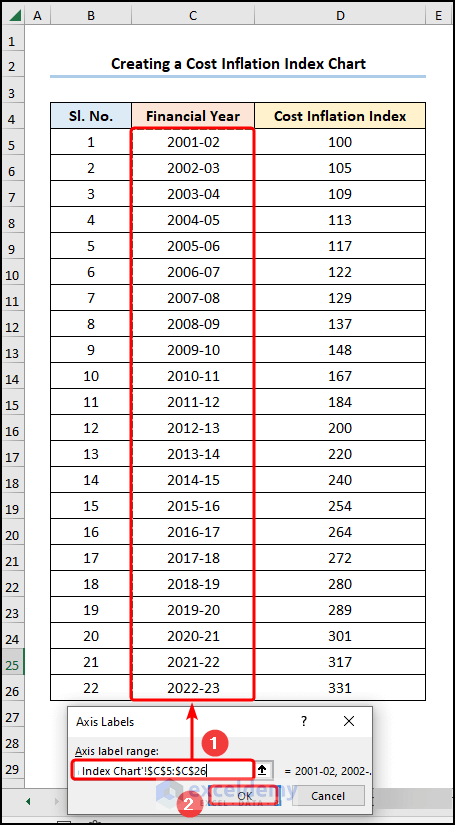
Not long after, select the C5:C26 cells as the horizontal axis labels >> press OK.

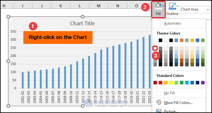
Later, right-click on the chart >> click on Fill >> choose a color, here we’ve chosen the “White, Background 1, Darker 5%” color.

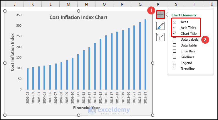
Eventually, format the chart using the Chart Elements option.

In addition to the default selection, enable the Axes Title to provide axes names. Here, it is the “Financial Year” and “Cost Inflation Index”.
Now, add the Chart Title, for example, “Cost Inflation Index Chart”.
Further, uncheck the Gridlines option to give your chart a clean look.

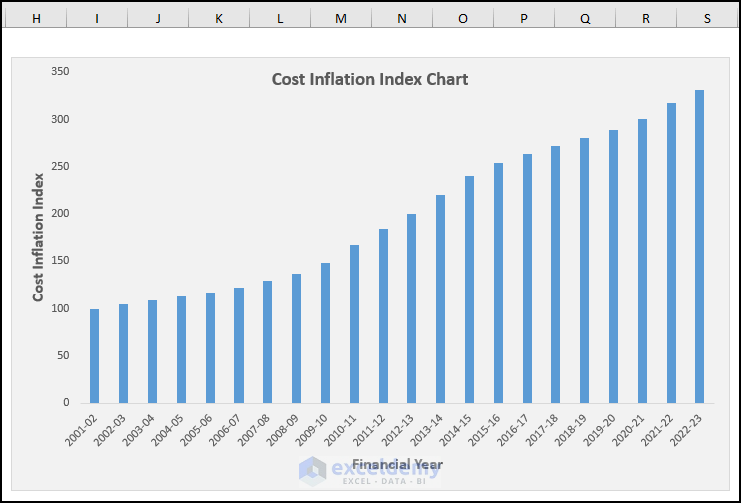
Subsequently, this should generate the chart as shown in the figure below.

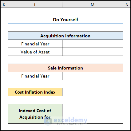
Practice Section

We have provided a Practice section on the right side of each sheet so you can practice yourself. Please make sure to do it by yourself.

Download Practice Workbook

Constructing Cost Inflation Index Calculator.xlsx

Conclusion

To sum up, we hope this article helps you understand the process of constructing a cost inflation index calculator in Excel. Now, if you have any queries, please leave a comment below.

<< Go Back to Cost Calculator | Finance Template | Excel Templates

Get FREE Advanced Excel Exercises with Solutions!