How to Create Cost of Delay Calculator in Excel (with Easy Steps)

Business analysts frequently have to choose which goods or projects to prioritize. There is a trade-off between projects, particularly about which project one should concentrate on first to start the project. The Cost of Delay Calculator is a really useful tool to use when making decisions of this nature because it shows you the project’s Cost of Delay. You can undoubtedly use Excel, once again to develop a Cost of Delay Calculator. In this article, I’m going to provide a thorough, step-by-step demonstration of how to make a Cost of Delay Calculator and explain the procedures so that you may utilize them whenever necessary.

Before going to the next phase, let’s have a look at the final output of what you are going to get.

What Is Cost of Delay Calculator?

If a project or product launches after the planned time frame, the Cost of Delay is the amount of money lost per unit of time. The Cost of Delay for the product “P” would be $10,000 per month, for instance, if you were preparing to launch a new product “P” in the market, and you ultimately launched the product one month later than you first anticipated, incurring a loss of $10,000.

Types of Cost of Delay

There are different types of Cost of Delay(CoD). I’m mentioning them briefly here.

Standard Curve: In standard CoD, the relationship between delay time and CoD is quite linear. This means, if the delay time increases, the CoD increases in a linear fashion. This is usually preferred to ease calculation.
Fixed Date Curve: This type of CoD works on a fixed deadline. And the rate of change of CoD is variable. Hence, the calculation of CoD is complicated as well. In short, there is a time when CoD will increase a lot and the value of CoD is not that much before or after that specific time period.
Intangible Curve: This applies for projects with low priority. The CoD is minimal here and the change is rare.
Urgent Curve: This is related to the projects with top priority. The CoD is huge in this case. That means, even a small delay in the project will result in a great loss.

How to Create Cost of Delay Calculator in Excel: with Easy Steps

In the following parts of this article, I’ll show you how to create a Cost of Delay Calculator in Excel. I’ll break down the full process into four steps so that you can visualize it clearly. I’ve used the Microsoft Excel 365 version for demonstration purposes. You may use your preferred version if needed.

Step 1: Creating Basic Particulars of Cost Analysis Data Set

In this section, let’s create a Data Set on which we’ll calculate the Cost of Delay. As we’ve stated earlier, we’ll show the full process in 4 simple steps and in the first step, we’ll create a table containing all the cost information. To prepare the Basic Particulars of Cost Analysis, we’ll create two tables following the steps described below.

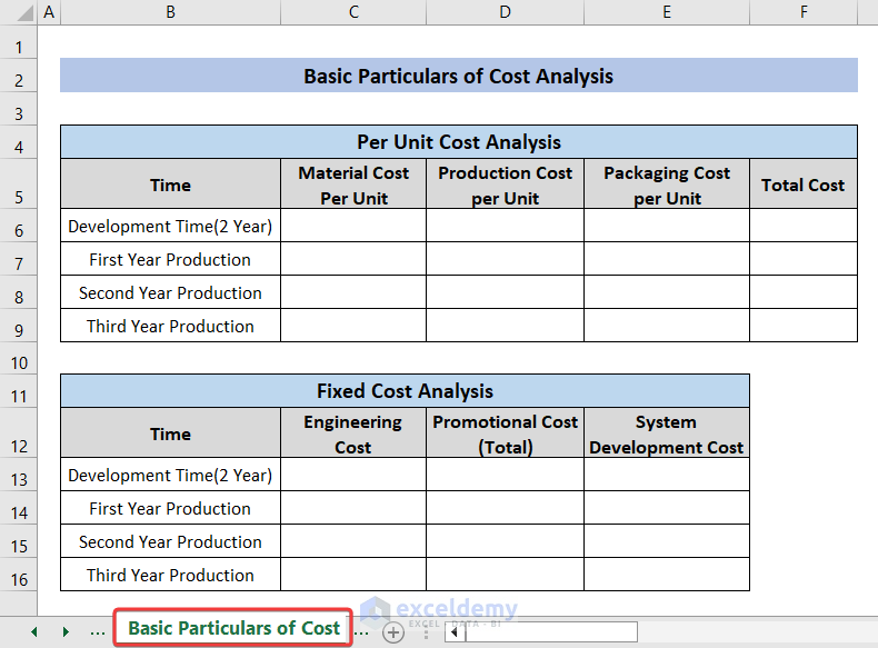
First of all, for a table titled Per Unit Cost Analysis creation, create columns titled Time, Material Cost per Unit, Production Cost per Unit, Packaging Cost per Unit and Total Cost in the B5:F5 We will create this table in the worksheet named Basic Particulars of Cost. Also, create another table named Fixed Cost Analysis with the headers named Time, Engineering Cost, Promotional Cost (Total) and System Development Cost.

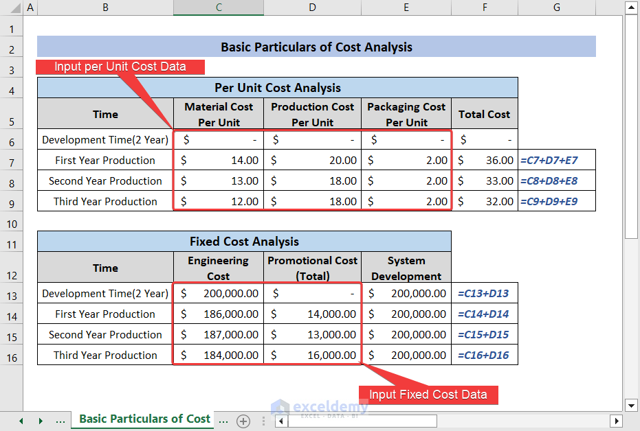
Now input the data and formulas in the corresponding cells to calculate the Total Cost and System Development
Note that the Total Cost is the summation of Material Cost, Production Cost and Packaging Cost per unit. So, the formula in cell F7 is =C7+D7+E7. Type this formula in cell F7 and press ENTER.
Similarly I’ve used =C8+D8+E8 formula in cell F8 and =C9+D9+E9 formula in cell F9.
Also, the System Development Cost is the summation of Engineering Cost and Promotional Cost(Total). So I’ve used =C13+D13 formula in cell E3. Press ENTER after writing this formula.
Similarly, I’ve used =C14+D14 in cell E14, =C15+D15 in cell E15 and =C16+D16 in cell E16 to calculate the respective System Development Cost.

Hence the data set for cost analysis is complete now.

Step 2: Calculating Profits According to Assumed Data Set

In this step, we’ll create a table for calculating Profit. Then, we’ll insert the corresponding cell values and use formulas to calculate the final profit. We’ll use this data for the final Cost of Delay calculation.

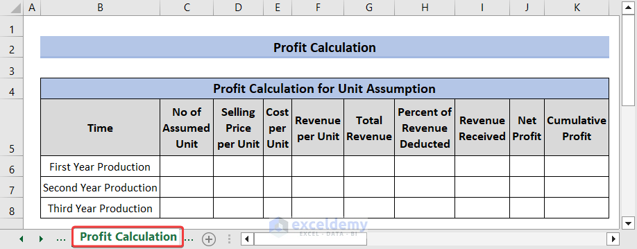
First of all, create columns titled Time, No of Assumed Unit, Selling Price per Unit, Cost per Unit, Revenue Per Unit, Total Revenue, Percent of Revenue Deducted, Revenue Received, Net Profit and Cumulative Profit in the B5:K8 We will create this table in the worksheet named Profit Calculation.

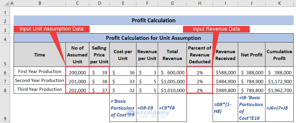
Now, input the following data and formulas in the corresponding cells for profit calculation.
I’ve used the formula =’Basic Particulars of Cost’!F7 in cell E6 to populate the Cost per Unit Type this formula in cell E6 and press ENTER. Similarly, the formula in cell E7 is =’Basic Particulars of Cost’!F8 and the formula in cell E8 is =’Basic Particulars of Cost’!F9.
The formula for calculating Revenue per Unit in cell F6 is =D6-E6. Press ENTER after typing this formula. Similarly, the formulas in cell F7 is =D7-E7 and in cell F8 is =D8-E8.
I’ve calculated Total Revenue in cell G6 using the formula =C6*F6. Press ENTER after typing the formula. Similarly, the formula in cell G7 is =C7*F7 and in cell G8 is =C8*F8.
To calculate the Revenue Received, I’ve used the formula in cell I6 is =G6*(1-H6). Press ENTER after typing the formula. Similarly, the formula in cell I7 is =G7*(1-H7) and in cell I8 is =G8*(1-H8).
I’ve typed the formula =I6-‘Basic Particulars of Cost’!E14 in cell J6 and pressed ENTER to get the Net Profit. Similarly, the formula in cell J7 is =I7-‘Basic Particulars of Cost’!E15 and in cell J8 is =I8-‘Basic Particulars of Cost’!E16.
Now we’ll calculate Cumulative Profit. The formula in cell K6 is =J6. Press ENTER after typing the formula. The formula in cell K7 is =J6+J7 and in cell K8 is =J6+J7+J8.

Hence the Profit Calculation for Unit Assumption is complete now.

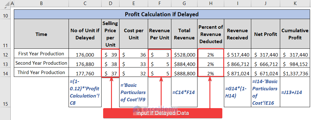
Step 3: Calculating Profits If Delay Happens

At this step, we are assuming that the product launched is delayed by one month. Therefore, it won’t be possible to produce 12% of the assumed unit.So the overall unit produced will be (1-0.12) times the unit assumed. Hence, Our Net Profit will be affected. As a result, Cost of Delay will appear.

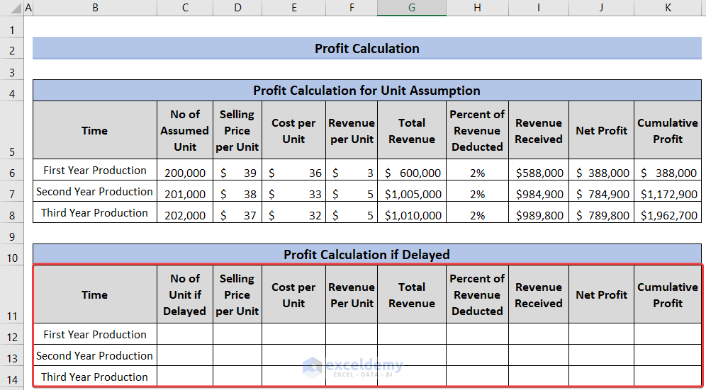
Create a table titled Profit Calculation if Delayed just like the table above titled Profit Calculation for Unit Assumption, except the second header(C11) will be titled as No of Unit if Delayed.

Now, insert the corresponding cell values and formulas as shown in the image to calculate the profit.
To calculate the No of Unit if Delayed, I’ve used the formula =(1-0.12)*’Basic Particulars of Cost’!C6 in cell C12. Type this formula in cell C12 and press ENTER.
Similarly, the formula in cell C13 is =(1-0.12)*’Basic Particulars of Cost’!C7 and the formula in cell C14 is =(1-0.12)*’Basic Particulars of Cost’!C8.
The formula to populate Cost per Unit in cell E12 is =’Basic Particulars of Cost’!F7.Press ENTER after typing the formula.
Similarly, the formula in cell E13 is =’Basic Particulars of Cost’!F8 and in cell E14 is =’Basic Particulars of Cost’!F9.
The formula to calculate Total Revenue in cell G12 is =C12*F12. Press ENTER after typing the formula. Similarly, the formula in cell G13 is =C13*F13 and in cell G14 is =C14*F14.
Use the formula in cell I12 is =G12*(1-H12) to get the value of Revenue Received. Press ENTER after typing the formula. Similarly, the formula in cell I13 is =G13*(1-H13) and in cell I14 is =G14*(1-H14).
To compute the Net Profit, I’ve typed the formula =I12-‘Basic Particulars of Cost’!E14 in cell J12 and pressed ENTER. Similarly, the formula in cell J13 is =I13-‘Basic Particulars of Cost’!E15 and in cell J14 is =I14-‘Basic Particulars of Cost’!E16.
Now we’ll calculate Cumulative Profit. The formula in cell K12 is =J12. Press ENTER after typing the formula. The formula in cell K13 is =J12+J13 and in cell K14 is =J12+J13+J14.

Hence, we’ll get all the data necessary to calculate the Cost of Delay.

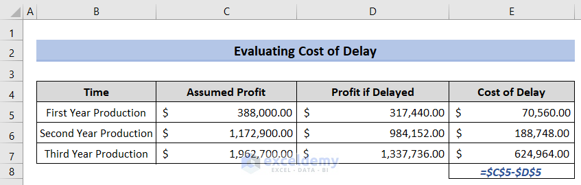
Step 4: Evaluating Cost of Delay

Now, we’re only one step behind to create the Cost of Delay Calculator in Excel. We need to create a table including the data to proceed our calculation. We’ll create this table in a new Worksheet named Cost of Delay.

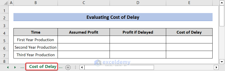
Create a table titled Evaluating Cost of Delay in cells ranging from B4 to E7. The table contains headers like Time, Assumed Profit, Profit if Delayed and Cost of Delay.

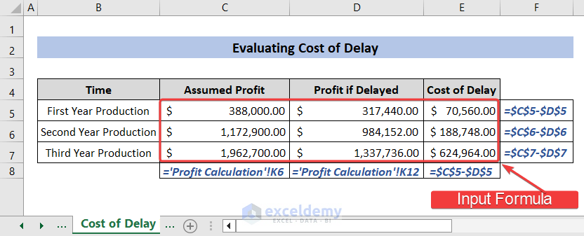
Insert the formulas in the corresponding cells to calculate Cost of Delay. I’ve used the formula =’Profit Calculation’!K6 in cell C5, =’Profit Calculation’!K12 in cell D5 to populate the respective values in the corresponding cells.
To calculate the CoD for the First Year Production, I’ve typed the =$C$5-$D$5 in cell E5 and pressed ENTER.I’ll get the CoD value now.
The rest of the CoD are calculated following this pattern.We can also use the Fill Handle to compute the rest of the CoD.

So, cells E5, E6 and E7 contain the Cost of Delay values for the first, second and third year production. This is visible that, The value increases significantly over the time.

How to Calculate CD3 Score to Prioritize Projects in Excel

CD3 score helps you prioritize projects. We can calculate the CD3 score dividing CoD by duration. For example, if we have a total of three projects named Project A, Project B and Project C. The time to develop these projects are 6, 8 and 12 months respectively. Also, the projects will generate a profit of 10,000 USD, 12000 USD and 22000 USD.

The dataset looks like this.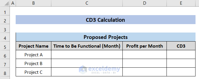

Now we need to calculate the CD3 values. The formula to do so is:
CD3=(Profit per Month/Time to develop Project/1000)

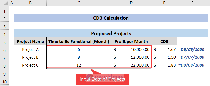
Type =D6/C6/1000 in cell F6 and press ENTER. This will give us the CD3 value for Project A.
Similarly use the formula =D7/C7/1000 in cell F7 and =D8/C8/1000 in cell F8. We’ll get all the CD3 values in this way.

We can see from the image that the value of CD3 is greatest for Project C. So, according to the concept of CD3, Project C should get top priority in terms of monetary value.

Takeaways from This Article

After thoroughly following this article, you should know:

Have a clear concept of what is the Cost of Delay Calculator and how to build it in Excel.
Be able to create and use the Cost of Delay Calculator of your own or reuse our Cost of Delay Calculator.
Get a functional idea of how to calculate CD3 value in Excel and how to use it.

Things to Remember

When you will work to build a Cost of Delay Calculator of your own using the method I’ve demonstrated in Excel, please keep in mind that:

Include all the no of years you are calculating CoD for in your dataset.
We’ve used worksheet references in our formulas. Please do accordingly when you’re using formulas and make necessary adjustments if needed.
Take care when you refer to any cell in the formulas.

Frequently Asked Questions

What are the benefits of using the Cost of delay Calculator?

The benefits of Cost of Delay Calculator are

The Cost of Delay Calculator helps to prioritize projects that are most important based on financial impact.
Reduce the mismanagement of allocating limited resources in projects. Thus, it brings out the most efficient way to save time and money.

Download Practice Workbook

You may download the Practice Workbook and practice yourself.

Cost of Dealy Calculator.xlsx

Conclusion

If you’re at this segment, I thank you for your interest in this content. I’ve demonstrated how to create a Cost of Delay Calculator in Excel. I’ve demonstrated a practical example of how you can use it in real life scenarios. I hope you get the necessary solution. Being said that, if you face any problem regarding this article or have any queries, please feel free to leave a comment in the comment box. Have a good day!

<< Go Back to Cost Calculator | Finance Template | Excel Templates

Get FREE Advanced Excel Exercises with Solutions!