Method 1 – Inserting VLOOKUP with a Helper Column to Compare Three Columns in Excel
Steps:
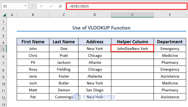
- Create a helper column.
- Go to E5 and insert the following formula
=B5&C5&D5- Press ENTER to get the output.
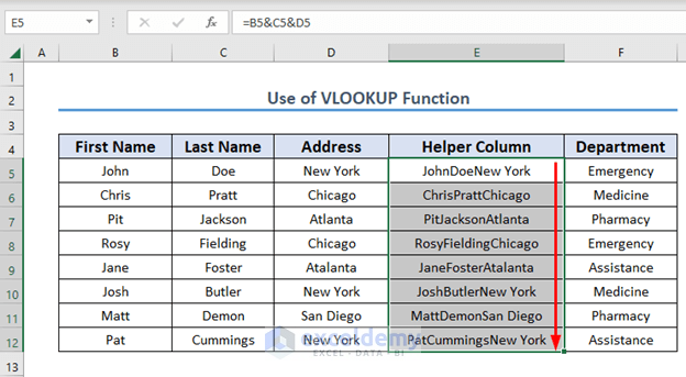
- Use Fill Handle to AutoFill up to E12.
- Copy any cell from the Helper Column and paste it to B17.
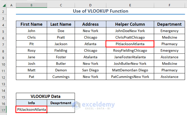
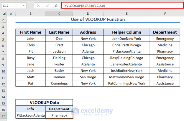
- Insert the following formula in C17.
=VLOOKUP(B17,E5:F12,2,0)- Press ENTER to get the output.
Formula Explanation
- The lookup_value is B17.
- The table_array is E5:F12. Excel will look for B17 in this array.
- The col_index is 2. That means, Excel will return the corresponding department name.
Method 2 – Applying the Ampersand Sign with Excel VLOOKUP to Compare Three Columns
Steps:
- Go to E17 and insert the following formula
=VLOOKUP(B17&C17&D17,$B$4:$E$12,4)- Press ENTER to get the output.
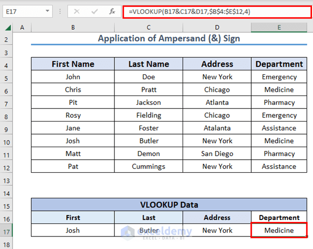
Formula Explanation
- The lookup_value is B17&C17&D17.
- The table_array is $B$4:$E$12. Excel will look for B17&C17&D17 in this array.
- The col_index is 4. That means, Excel will return the corresponding department name.
Method 3 – Using Excel VLOOKUP-MATCH Formula to Compare Three Columns
Steps:
- Go to D17 and insert the following formula
=VLOOKUP(B17,$B$5:$E$12,MATCH(C17,B4:E4,0),0)- Press ENTER to get the output.
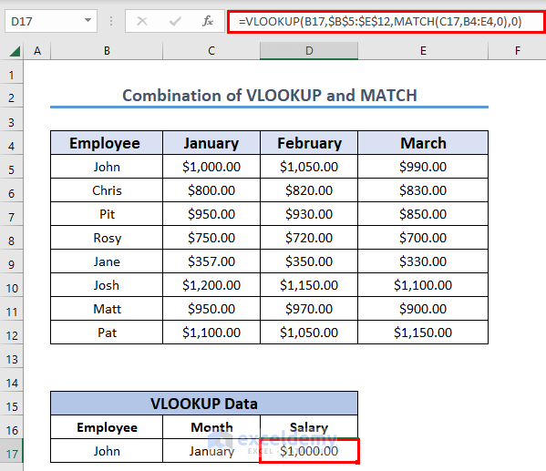
Formula Breakdown
- MATCH(C17,B4:E4,0) → This indicates the col_index for the VLOOKUP function.
- Output: 2.
- VLOOKUP(B17,$B$5:$E$12,MATCH(C17,B4:E4,0),0) → This becomes,
- VLOOKUP(B17,$B$5:$E$12,2,0)
- Output: 1000
How to Combine INDEX and MATCH Functions to Compare Three Columns in Excel
Steps:
- Go to E17 and insert the following formula
=INDEX(E5:E12,MATCH(1,(B5:B12=B17)*(C5:C12=C17)*(D5:D12=D17),0))- Since this is an array formula, press CTRL + SHIFT + ENTER to get the output.
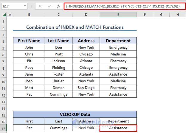
Formula Breakdown
- (B5:B12=B17)*(C5:C12=C17)*(D5:D12=D17) → This is the lookup_array for the MATCH function.
- Output: {0;0;0;0;0;0;0;1}
- MATCH(1,(B5:B12=B17)*(C5:C12=C17)*(D5:D12=D17),0) → This is the row_num for the INDEX function.
- Output: 8
- INDEX(E5:E12,MATCH(1,(B5:B12=B17)*(C5:C12=C17)*(D5:D12=D17),0)) → This becomes,
- INDEX(E5:E12,8)
- Output: Assistance
Notice the curly bracket {} in the formula bar. It indicates an array formula.
Download the Practice Workbook
<< Go Back to Columns | Compare | Learn Excel
Get FREE Advanced Excel Exercises with Solutions!

Thanks Maruf, very useful information
Hello Mohammad,
You are welcome.
Regards
ExcelDemy