How to Create Common Size Balance Sheet in Excel (3 Simple Steps)

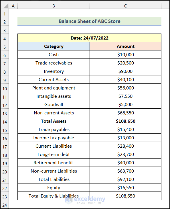
We have the Balance Sheet of ABC Store as our dataset. We’ll create a common-size balance sheet for this dataset.

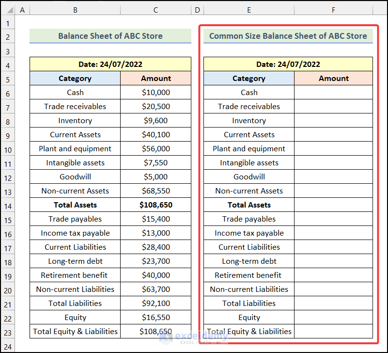
Step 1 – Create a New Table

• Create an identical table just like the dataset. Keep the Amount column blank as shown in the following picture.

Read More: How to Make Automatic Balance Sheet in Excel

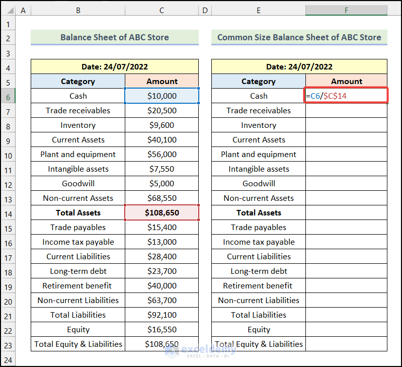
Step 2 – Calculate the Relative Percentage

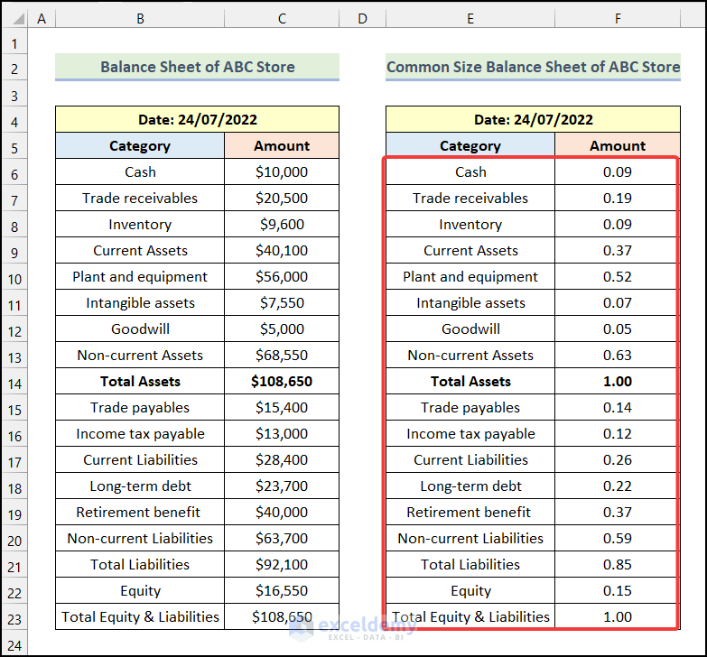
• Enter the following formula in cell F6.

Cell C6 represents a cell of the Category column, and cell $C$14 refers to the cell of Total Assets.

• Press Enter.

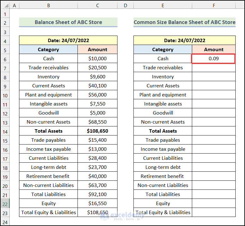
The relative percentage of Cash will be displayed in cell F6 as marked in the following image.

• Use the AutoFill option to get the remaining outputs.

Read More: How to Make a Forecasting Balance Sheet in Excel

Step 3 – Format the Output Table

• Select the cells in the output column.
• Go to the Home tab from Ribbon.
• Click on the Number Format drop-down.
• Select the Percentage option from the drop-down.

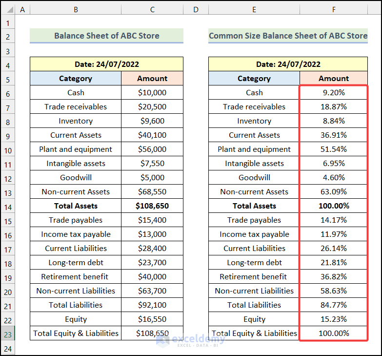
Alternatively, you can multiply 100 by the inserted formula in Excel. The adjusted formula for the F6 will be-

The cells of the output column will be formatted as percentage values as shown in the following picture.

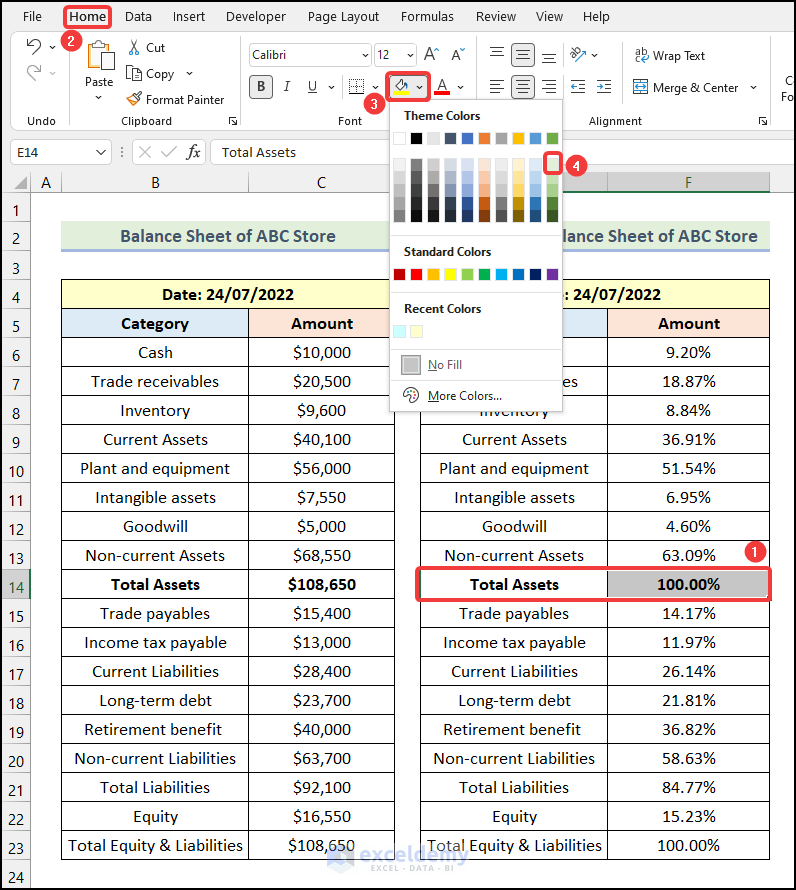
• Select the cells E14 and F14.
• Go to the Home tab from Ribbon.
• Click on the Fill Color drop-down.
• Choose your preferred color from the drop-down.

Consequently, you will have the common-size balance sheet like in the following image.

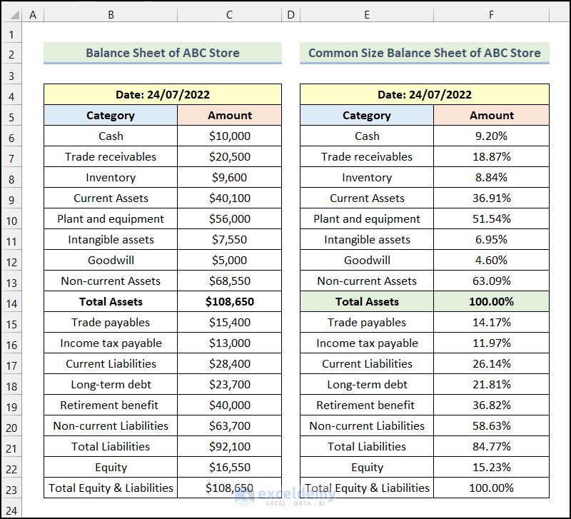
Note: Here, the cell of the relative percentage of Total Assets works as an identifier. If its value is 100%, that will mean that we have done the calculations correctly.

Read More: Rental Property Balance Sheet in Excel

How to Create Common-Size Income Statements in Excel

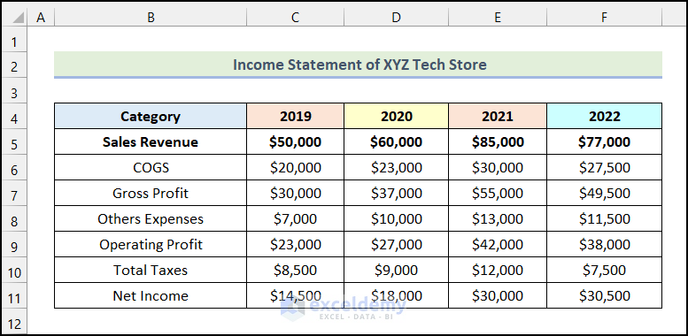
We have the Income Statement of XYZ Tech Store for 4 years. We’ll create a common-size income statement with this dataset.

Steps:

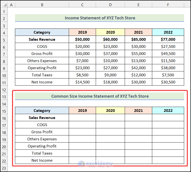
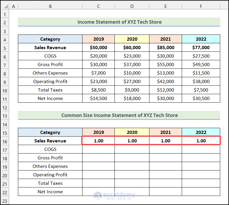
• Create a table as shown in the following image, with emptied out values.

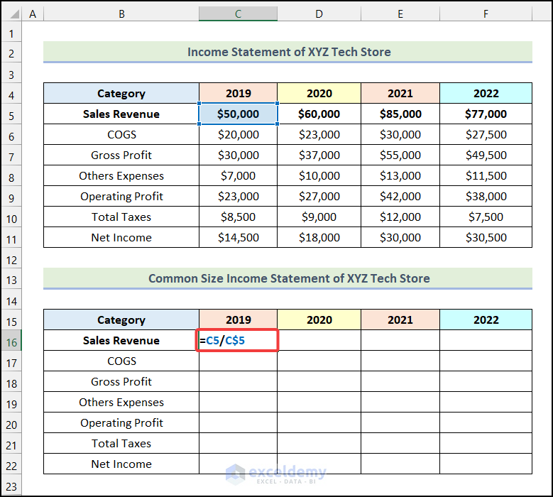
• Enter the following formula in cell C16.

Here, cell C5 represents the Sales Revenue for the year 2019.

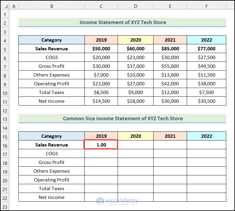
• Press Enter.

Note: For the denominator, we only locked the row number (C$5). We will be able to drag this formula both horizontally and vertically.

You will have the relative percentage of Sales Revenue for the year 2019.

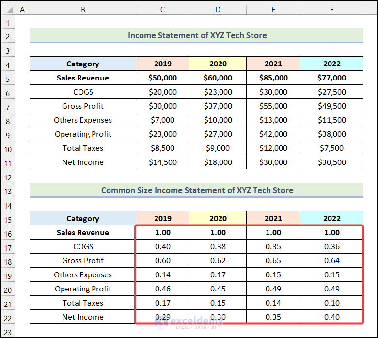
• Drag the Fill Handle in the row direction up to cell F16 and you will get the following outputs.

• By using the AutoFill feature of Excel, you can get the remaining outputs as demonstrated in the following picture.

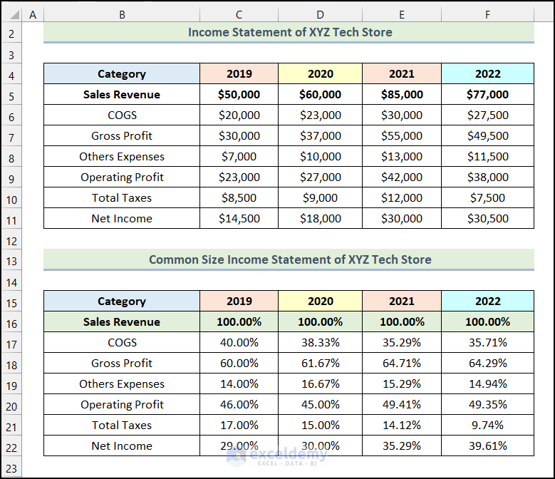
• Format the values as percentages.

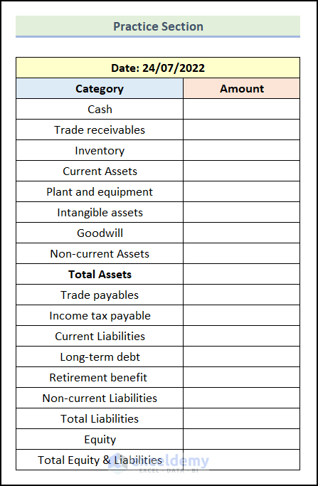
Practice Section

In the Excel Workbook, we have provided a Practice Section on the right side of the worksheet.

Click on the image for better quality<\em>

Download the Practice Workbook

<< Go Back to Balance Sheet | Finance Template | Excel Templates