This tutorial illustrates three easy methods to calculate the weighted average in Excel. While evaluating a simple average of a group of numbers, we assume that each value has the same weight or importance. However, it’s not so simple all the time. Among a variety of tasks, some are always more significant than others. And that’s the case when we need to calculate the weighted average.
What Is Weighted Average in Excel?
Weighted average in Excel refers to the arithmetic mean where certain data elements are always more important than others. If we say it in another way, every value that we will average has a specific weight.
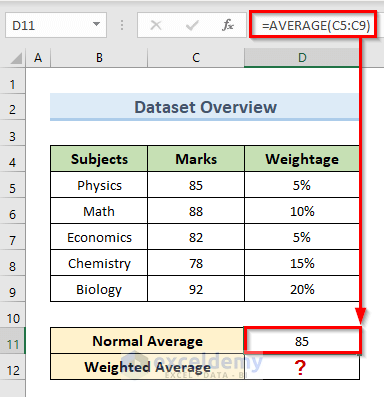
From the following dataset, we can see the marks of a student in different subjects. But all the subjects do not carry the same significance. That’s why we have a column named Weightage to measure the importance of each subject. Use the following AVERAGE formula in cell C11:
=AVERAGE(C5:C9)The above formula returns the value of the Normal Average in cell C11. In the image, we can see that the value is 85.
Now, we will calculate the weighted average and will see its difference from the normal average.
How to Calculate Weighted Average in Excel: 3 Easy Methods
To demonstrate the three methods to calculate the weighted average in Excel, we will use the SUM and SUMPRODUCT functions. We can calculate the weighted average by using normal mathematical formulas but the use of Excel functions makes it more convenient. To make you understand better, we will use the same dataset to explain all the methods.
1. Calculate Weighted Average with Generic Formula in Excel
First and foremost, we will use the generic weighted average to calculate the weighted average from our dataset.
Generic Formula:
Weighted Average = (Sum of Weighted Terms)/(Total Number of Terms)
Let’s see the steps to use this formula in the following dataset.
STEPS:
- To begin with, select cell D12.
- In addition, type the following formula in that cell:
=(C5*D5+C6*D6+C7*D7+C8*D8+C9*D9)/(D5+D6+D7+D8+D9)
- Now, press Enter.
- Finally, we can see the result in the following image.

2. Estimate Weighted Average with Excel SUM Function
In the second method, we will use the SUM function to estimate the weighted average in Excel. The SUM function in Excel returns the total of supplied values. Follow the below steps to perform this method.
STEPS:
- First, select cell D12.
- Next, insert the following formula in that cell:
=SUM(C5:C9*D5:D9)/SUM(D5:D9)
- Then, press Enter.
- In the end, we get the value of the weighted average in cell D12.

3. Combine SUMPRODUCT & SUM Functions to Calculate Weighted Average in Excel
In the last method, we will combine the SUMPRODUCT and SUM functions to calculate the weighted average in Excel. The SUMPRODUCT functionin Excel calculates the sum of the products of two or more ranges or arrays. By default this function does multiplication. But we can also do addition, subtraction, and division. To use these functions to calculate the weighted average we will follow the below simple steps.
STEPS:
- Firstly, select cell D12.
- Secondly, write down the following formula in that cell:
=SUMPRODUCT(C5:C9,D5:D9)/SUM(D5:D9)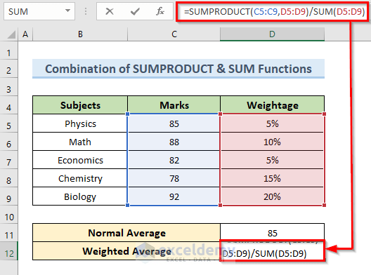
- Press, Enter.
- Lastly, We get our desired value of the weighted average in cell D12.

Things to Remember
- While using the SUMPRODUCT function we have to use all the array arguments in the same size. Otherwise, the function will return #VALUE! Error.
- The SUMPRODUCT function evaluates zeros if the datasets contain text data in a range.
Download Practice Workbook
You can download the practice workbook from here.
Conclusion
In conclusion, this tutorial shows three easy and effective methods to calculate the weighted average in Excel. Use the practice worksheet added to this article to put your skills to the test. If you have any questions, please leave a comment in the box below. We’ll do our best to respond as soon as possible. Keep an eye on our website for more interesting Microsoft Excel solutions in the future.
Get FREE Advanced Excel Exercises with Solutions!
